pak::pak(c("microbenchmark", "tictoc", "dtplyr", "duckplyr", "mirai", "furrr"))24 Making R Faster 🚀
Class Objectives
- Measure your code’s speed – Know exactly how fast (or slow) your code is running
- Parallel computing – Use multiple CPU cores for CPU-heavy tasks
- Faster data wrangling – Know when swapping tidyverse functions for faster engines under the hood is (and is not) worth it.
Packages for this chapter
If you haven’t installed the following packages, run this code:
R sometimes gets a bad rap for being slower than languages like C++ or Julia. That’s partly true: if you are really serious about performance, you might want to learn another language. However, you can often make R much faster without rewriting your code or learning a new language.
Let’s start by loading tidyverse and a dataset from the nycflights13 package which has more than 330,000 rows.
library(tidyverse)
data(flights, package = "nycflights13")
Note that we are not using the tidylog package this time. tidylog prints a message summarising each verb so that you know what happens in each step. This is great for understanding what the code is doing, but it slows down the execution.
24.1 Figure Out How Fast Your Code Is
24.1.1 Quick Check with tictoc
The tictoc package (no relation to social media platform) lets you time code chunks easily:
library(tictoc)
tic()
model_r2 <- flights |>
group_by(carrier, origin) |>
nest() |>
mutate(r2 = map_vec(data, \(x) summary(lm(arr_delay ~ dep_delay, data = x))$r.squared))
toc()- 1
- Start the timer!
- 2
-
Your code goes in between
tic()andtoc(). - 3
- Stop the timer and print the time
0.948 sec elapsed24.1.2 Compare Methods with microbenchmark
Want to test multiple approaches? microbenchmark runs code repeatedly and compares results. Here we compute the squares of 1 to 100,000 in three ways: a loop that grows a vector, a loop with a preallocated vector, and a vectorized expression:
library(microbenchmark)
n <- 1e5
benchmark <- microbenchmark(
growing = {
z <- c()
for (i in 1:n) z[i] <- i^2
},
preallocated = {
z <- numeric(n)
for (i in 1:n) z[i] <- i^2
},
vectorized = (1:n)^2,
times = 10
)
print(benchmark)- 1
-
Name the method on the left and the code on the right. This loop grows
zat every iteration. - 2
-
Same loop, but
zis created with its final length first. - 3
- No loop at all.
- 4
- Run each code 10 times
- 5
-
Print the time it took to run each method (pay attention to the
unitin the header of the table)
Unit: microseconds
         expr       min        lq       mean    median        uq       max
      growing 10586.036 11099.807 12189.1114 12100.412 13545.088 13788.546
 preallocated  2705.549  2761.473  3285.5391  2846.794  3555.110  5005.280
   vectorized    93.562   157.768   174.4345   175.398   179.129   252.437
 neval cld
    10 a
    10  b
    10   c
How to read the table: compare the median column, and look at the cld column, where methods sharing a letter are not clearly different. Growing the vector is clearly the slowest, and preallocating already helps a lot. The vectorized version has the smallest median, by a wide margin (the cld letters only group methods that are statistically indistinguishable, which is a coarse comparison, so always look at the medians too). Note that a benchmark only tells you something when the methods actually differ in what they do: when the run time is dominated by one expensive step (such as fitting many lm() models), different ways of looping over it will perform about the same.
It might be helpful to visualize the results. You can use the autoplot function to do this easily.
autoplot(benchmark)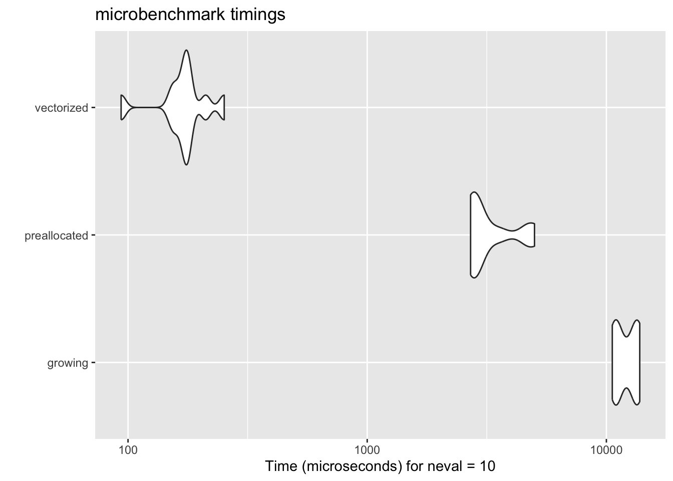
24.1.3 Estimate how long it will take to run your code
A great new feature in purrr is the introduction of .progress argument. This allows you to estimate how long it will take to run your code.
As the codes above runs very fast, we use a more time-consuming task (just for illustration purposes).
tibble(x = 1:500) |>
mutate(y = map_dbl(x, \(x) {
Sys.sleep(0.01)
x
},
.progress = TRUE))- 1
- Sleep for 0.01 seconds
- 2
- Show a progress bar
24.2 Parallel Computing
R usually uses one CPU core. But most computers have several cores! By sending independent tasks to multiple cores, you can get speedups with only a small change to your code (as long as the tasks are heavy enough to be worth the coordination).
24.2.1 furrr: A single command change
Before mirai was integrated into purrr, the standard approach was the furrr package. You may still see this in older code. The idea is the same: replace map with future_map and set a plan.
library(furrr)
plan(multisession, workers = 4)

tic()
model_r2 <- flights |>
  group_by(carrier, origin) |>
  nest() |>
  mutate(r2 = future_map_dbl(data, \(x) summary(lm(arr_delay ~ dep_delay, data = x))$r.squared))
toc()

plan(sequential) # go back to running on one core
We can also add a progress bar. (This is only a demo of the progress bar: with 10,000 tiny tasks, the overhead of sending them to workers will likely dominate, so do not expect a speedup.)
tibble(
    x = 1:10000
)  |>
    mutate(y = future_map(x, \(x) Sys.sleep(0.001),
               .progress = TRUE))

plan(sequential)
24.2.2 Built-in parallelism with mirai
Since purrr 1.1.0, parallel computing is built right into the map functions via the mirai package. The syntax change is minimal: just wrap your function with in_parallel() and set up mirai::daemons() beforehand.
To see a clear speedup, we want a task that is computationally heavy but does not require transferring large datasets between processes (since transferring data to background workers adds serialization overhead). Let’s simulate rolling two dice 20,000 times to check the probability of sum = 7, and repeat this simulation 100 times:
library(mirai)
parallelly::availableCores()
# 1. Sequential run
tic()
res_seq <- map_dbl(rep(20000, 100), \(n) {
mean(replicate(n, sum(sample(1:6, 2, replace = TRUE)) == 7))
})
toc()
# 2. Parallel run
daemons(max(1, parallelly::availableCores() - 1))
tic()
res_par <- map_dbl(rep(20000, 100),
in_parallel(\(n) {
mean(replicate(n, sum(sample(1:6, 2, replace = TRUE)) == 7))
}))
toc()
daemons(0)- 1
- Check how many cores are available
- 2
- Set the number of daemons (workers). We leave one core for the main process.
- 3
-
Wrap the function with
in_parallel()— that’s it! - 4
- Reset daemons when done
The key idea: in_parallel() is a function wrapper that signals purrr to run the function across multiple cores. It also ensures your function is self-contained and properly packaged to be sent to parallel processes. If daemons() is not set, it falls back to sequential processing — so your code never breaks.
Note: Parallelizing adds some overhead (think of the leader needing time to coordinate the workers and serialize data). Thus, it may cost more time than the non-parallelized version for small datasets or quick calculations.
24.3 Swap Tidyverse for Speed Demons
Another option is to keep writing dplyr-style code but let a faster engine run it. Be realistic, though: on a dataset of 330,000 rows, dplyr is already fast, and these tools mostly pay off with millions of rows or many repeated operations.
data.table is fast but has a steep learning curve. dtplyr lets you write tidyverse code that gets translated to data.table behind the scenes:
library(dtplyr)
flights |>
lazy_dt() |>
group_by(carrier, origin, year) |>
summarise(mean_arr_delay = mean(arr_delay, na.rm = TRUE)) |>
as_tibble()- 1
- Convert the tibble to a data table
- 2
-
Use all the
dplyrfunctions you know - 3
- Convert the data table back to a tibble
Is it faster here? Let’s check with microbenchmark:
microbenchmark(
  dplyr = flights |>
    group_by(carrier, origin) |>
    summarise(mean_arr_delay = mean(arr_delay, na.rm = TRUE), .groups = "drop"),
  dtplyr = flights |>
    lazy_dt() |>
    group_by(carrier, origin) |>
    summarise(mean_arr_delay = mean(arr_delay, na.rm = TRUE)) |>
    as_tibble(),
  times = 20
)
On this dataset the two are about the same (compare the medians and the cld letters, if shown): the gain only shows up with much larger data.
DuckDB is a fast database engine, which works well if you have a lot of data (like millions of rows). duckplyr is a package that translates dplyr code to duckdb code behind the scenes. So again, you can write as usual and do not need to worry about the underlying heavy machinery.
When you load the package, the messages clearly tell you that the dplyr methods are overwritten. We do not run this chunk here, because loading duckplyr changes how dplyr behaves for the rest of the session.
library(duckplyr)

flights |>
  group_by(carrier, origin, year) |>
  summarize(mean_arr_delay = mean(arr_delay, na.rm = TRUE))
24.4 Additional Resources
Making code faster is a very broad topic. Here are some additional resources that you need even more speed:
All of these packages are under active development, and it is hard to say which one is the best (they all have their own strengths). Some of them (like tidypolars) follow the dplyr grammar, while others (like collapse, with functions such as fsum() and fgroup_by()) have their own API, so the learning curve varies.
24.5 Remember: Speed Isn’t Everything! 🛑
Premature optimization is the root of all evil. – Donald Knuth
Only optimize code that’s slow enough to annoy you. Focus on correctness and readability first!