15 Other Types of Plots

Packages for this chapter

If you haven’t installed the following packages, run this code:

pak::pak(c("maps", "sf", "rnaturalearth", "rnaturalearthdata", "ggrepel", "viridis", "statebins", "tidygraph", "ggraph", "ape", "bioc::ggtree"))

In addition to the most common plots we’ve covered so far, many specialized plot types can be extremely useful depending on your research focus. While these plots may not be applicable to every project, they offer powerful ways to visualize complex data in specific fields.

15.1 Network plots

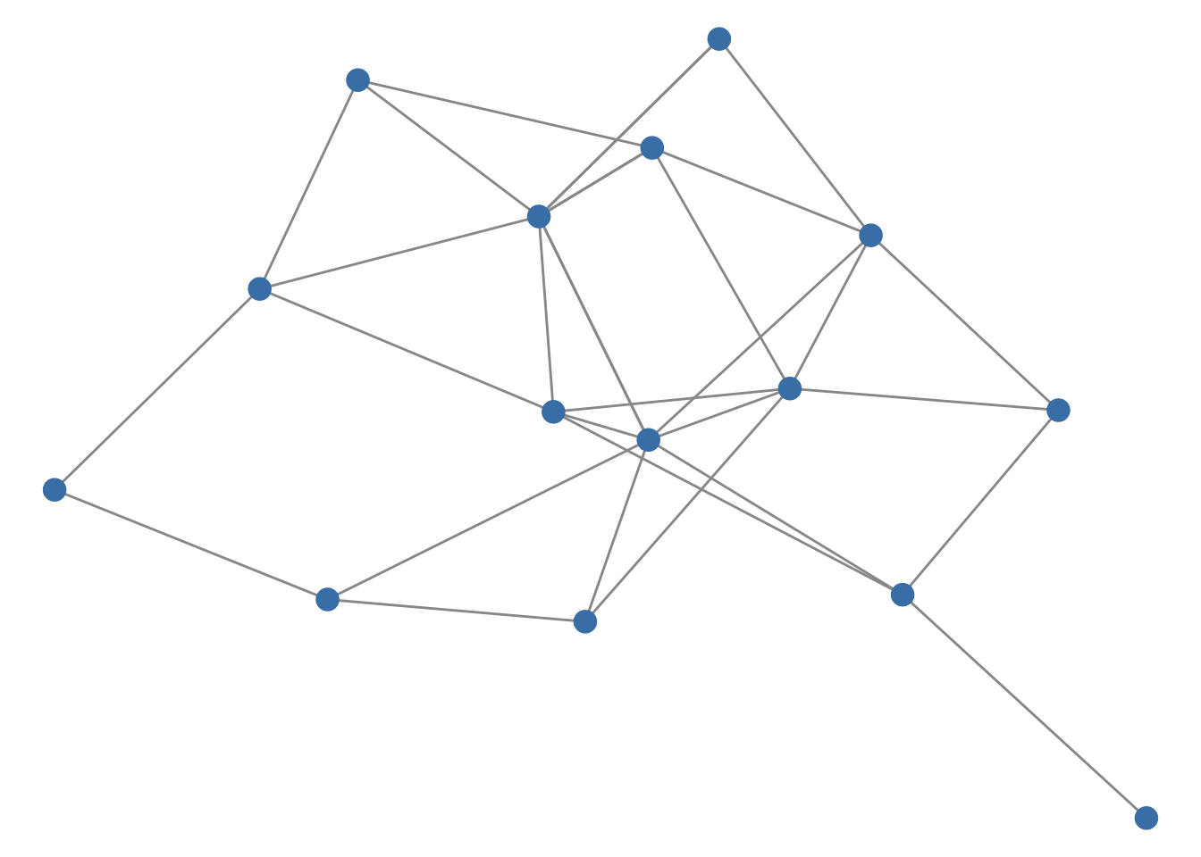
Networks are increasingly common. For example, ecological networks. With the power of the tidygraph package to structure your data and ggraph to render it beautifully, you can create visualizations that are both informative and striking. Here is a minimal example with a small random graph:

library(tidygraph)
library(ggraph)

set.seed(1)
play_erdos_renyi(n = 15, p = 0.15) |>
    ggraph(layout = "fr") +
    geom_edge_link(color = "grey60") +
    geom_node_point(size = 4, color = "steelblue") +
    theme_void()

1: Simulate a random graph with 15 nodes as a tidygraph object.
2: Compute a force-directed layout.
3: Draw the edges.
4: Draw the nodes.

For a look at what’s possible, check out these impressive examples here.

15.2 Phylogenetic trees

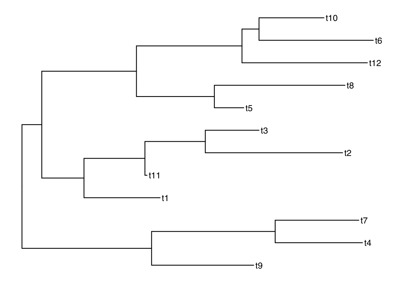
For researchers in evolutionary biology, phylogenetic trees are essential for illustrating evolutionary relationships. The ggtree package (from Bioconductor, hence the bioc:: prefix in the install code above) simplifies the process of creating detailed and informative trees. Here is a minimal example with a random tree from the ape package:

library(ggtree)

set.seed(1)
ape::rtree(12) |>
    ggtree() +
    geom_tiplab()

1: Simulate a random tree with 12 tips.
2: Draw the tree; ggtree() works like ggplot(), so you can add layers with +.
3: Label the tips.

To see more examples and learn more about its capabilities, visit here.

15.3 Spatial data

Spatial data visualization allows you to create maps and geospatial plots, providing visually compelling representations of data tied to geographic locations. This tutorial introduces the basics of creating maps using ggplot2, first with polygon data from the maps package and then with the sf package. While spatial data analysis is a vast topic, hopefully this guide provides a foundation for getting started.

15.3.1 Getting Started: Essential Packages

We’ll use a new package sf, a modern package for handling spatial data in R. It represents geographic features (like points, lines, and polygons) in a way that ggplot2 understands through geom_sf() (see the end of this section). We also use maps, which provides simple map data as ordinary data frames.

library(tidyverse)
library(sf)
library(maps)

1: Deal with spatial data
2: Load the map data package

Let’s start by creating a simple world map.

world_map <- map_data("world")

ggplot(world_map, aes(x = long, y = lat, group = group)) +
    geom_polygon(fill = "lightgray", colour = "white") +
    theme_void()

1: Load Map Data: The maps package provides pre-built map data. We’ll use map_data(“world”) to get a data frame representing the world’s countries.
2: Use longitude and latitude to plot the map
3: Plot with geom_polygon: ggplot2’s geom_polygon is used to draw shapes, which in this case are the country outlines. We need to tell it how the points are connected to form the polygons using the group aesthetic.
4: Clean Up with theme_void: theme_void() removes axis lines, labels, and the background, giving us a clean map.

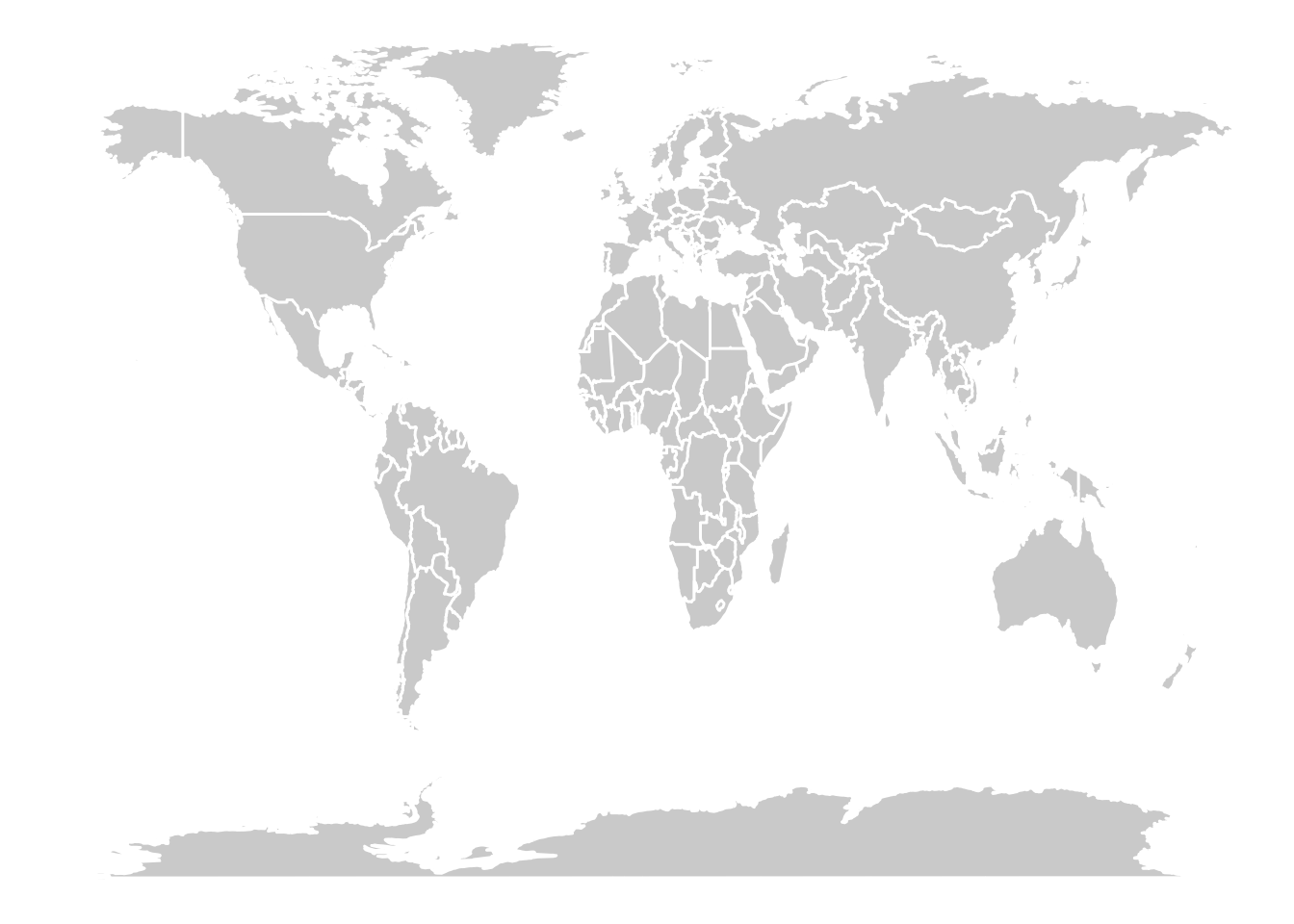
The map looks stretched because one degree of longitude and one degree of latitude are not the same distance. Adding coord_quickmap() (or coord_fixed()) fixes the aspect ratio approximately.

We can easily create maps of specific regions by filtering the world map data.

# Retrieve the map data for some Asian countries
some_asia_maps <- map_data("world", region = c(
  "Malaysia",
  "Philippines",
  "Thailand",
  "Vietnam"
))

# Calculate an approximate label position for each country
# (the mean of the polygon vertices, not a true centroid)
asia_lab_data <- some_asia_maps |>
  group_by(region) |>
  summarise(long = mean(long), lat = mean(lat))

# Plot the map
ggplot(some_asia_maps, aes(x = long, y = lat)) +
  geom_polygon(aes( group = group, fill = region))+
  ggrepel::geom_text_repel(aes(label = region), data = asia_lab_data,  size = 3)+
  scale_fill_viridis_d()+
  coord_quickmap()+
  theme_void()+
  theme(legend.position = "none")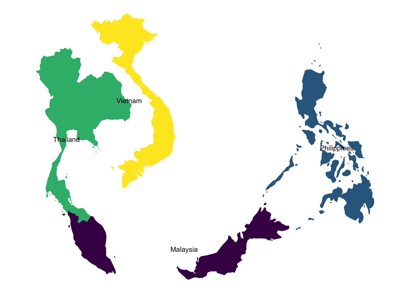

Because the label positions are just the average of the polygon vertices, they can land off-center or even in the sea for countries made of many islands (such as the Philippines). A true centroid, for example from sf::st_centroid(), is more reliable.

15.3.2 Mapping Data onto a Map

Now, let’s combine a map with external data. We’ll use the USArrests dataset and visualize assault arrest rates (arrests per 100,000 residents, 1973) across US states.

arrests_map <- USArrests  |> 
    as_tibble(rownames = "state")  |> 
    mutate(region = tolower(state))  |> 
    right_join(map_data("state"), by = "region")  

arrests_map  |> 
    ggplot(aes(long, lat, group = group))+
    geom_polygon(aes(fill = Assault), color = "white")+
    scale_fill_viridis_c(option = "D")+
    theme_void()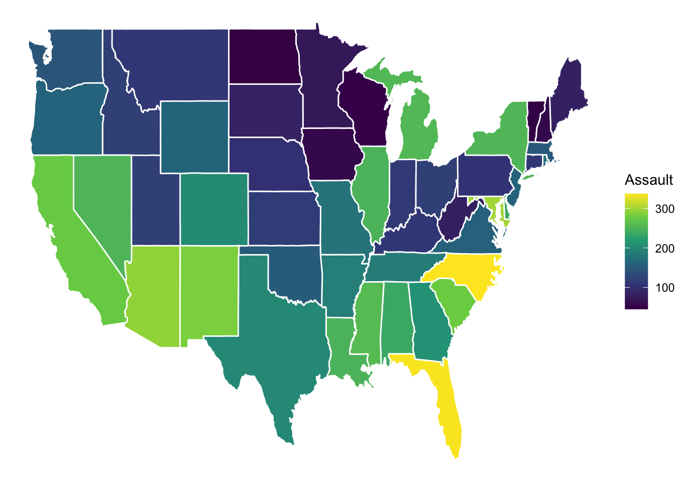

Importantly, a map does not always need to be geographically accurate. We can use the statebins package to make a useful visualization, giving every state a tile of equal size. Here we use the original USArrests table (one row per state) rather than the polygon table.

library(statebins)

USArrests |> 
    as_tibble(rownames = "state") |> 
    ggplot(aes(state = state, fill = Assault))+
    geom_statebins(color = "white")+
    scale_fill_viridis_c(option = "D")+
    theme_void()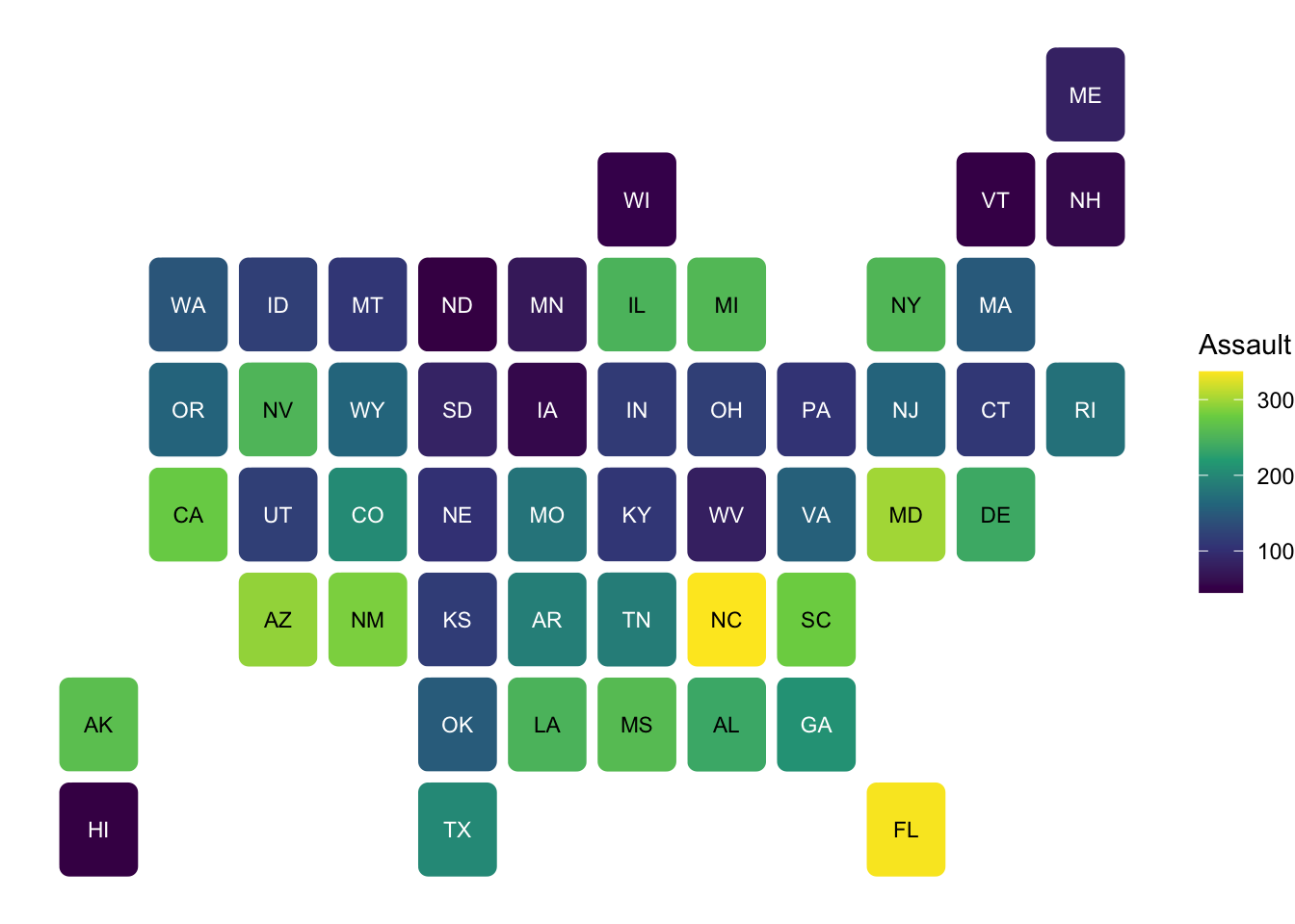

15.3.3 Maps with `sf`

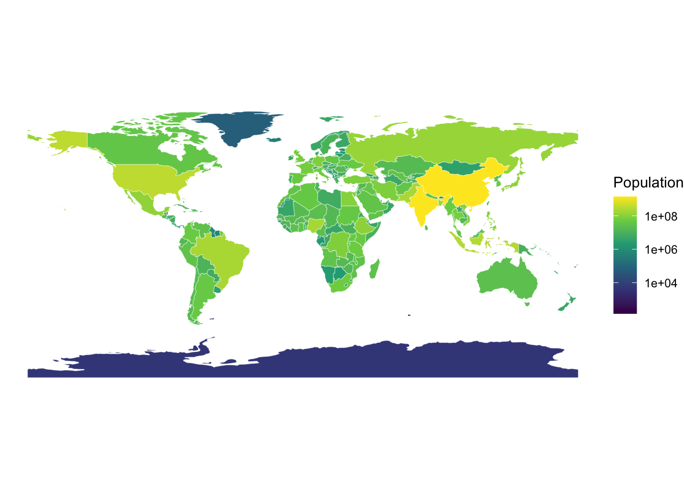
With sf, a map is a data frame with a special geometry column, and geom_sf() draws it directly, with no need for group or long/lat. Here we get country boundaries from the rnaturalearth package (the data are included in rnaturalearthdata, so no internet connection is needed).

world_sf <- rnaturalearth::ne_countries(scale = 110, returnclass = "sf")

world_sf |> 
    ggplot() +
    geom_sf(aes(fill = pop_est), color = "white", linewidth = 0.1) +
    scale_fill_viridis_c(trans = "log10", name = "Population") +
    theme_void()

1: Load low-resolution country boundaries as an sf object.
2: geom_sf() finds the geometry column automatically.
3: Fill by population estimate on a log scale, since populations vary by orders of magnitude.

15.3.4 Further Exploration

If you want to learn more about mapping, here are some useful packages:

ggmap: For using map tiles from online providers as your base map. Some providers require an API key (and some require billing), so check the ggmap tutorial for the currently supported services.
ggspatial: Provides tools for adding annotations like scale bars and north arrows to your maps.

Additionally, you can learn a lot from well-documented examples. Check out the following website for some outstanding examples with codes here.

15.1 Network plots

15.2 Phylogenetic trees

15.3 Spatial data

15.3.1 Getting Started: Essential Packages

15.3.2 Mapping Data onto a Map

15.3.3 Maps with sf

15.3.4 Further Exploration

15.3.3 Maps with `sf`