print("Hello, World!")- 1
-
The
print()function displays the text within on the console.
[1] "Hello, World!"Let’s begin at the most logical starting point: getting the software installed. To get started, I recommend this comprehensive installation guide that will walk you through the process seamlessly.
Think of R as a high-performance engine—capable of incredible feats but not particularly user-friendly on its own. RStudio is the sleek vehicle that lets you harness that power efficiently. While you could interact with R through a basic terminal, RStudio’s interface smoothly handles the otherwise clunky commands and makes certain tasks—like visualizing results or managing code—remarkably more accessible.
For this course, we will use RStudio as our primary IDE. It is an incredibly well-designed piece of software that makes your life easier when working with R (and Python). We’ll explore many of its features as we progress, starting with making your R code look better.
Positron is a next-generation IDE developed by the same team behind RStudio (Posit). Think of it as the modern evolution of RStudio—it keeps the familiar R-centric workflow but runs on a more powerful, extensible foundation. Students are welcome to use Positron instead of RStudio for this course; everything we cover will work in both.
VSCode is another popular, general-purpose IDE that supports R (and many other languages). It’s free, open-source, and highly extensible. Personally, I use VSCode for most of my R programming work.
One of the subtle joys of programming is crafting code that’s not only functional but also aesthetically pleasing. To enhance the readability of your R scripts, consider installing the Fira Code font. Instruction can be found here and here.
Another way to make your code more readable is to format the codes according to the tidyverse style guide. Of course, no one wants to memorize all. Luckily, you can use the styler package to do this as an addin in RStudio (link).
In the grand tradition of programming tutorials, let’s start with the classic “Hello, World!”—a humble beginning to our journey with R.
print("Hello, World!")print() function displays the text within on the console.
[1] "Hello, World!"Next, you can use R as a straightforward calculator:
3 + 2[1] 5You can also store results in variables (so you can use them later):
x <- 3 + 2
x3 + 2 to the variable x.
x displays the value of x on the console.
[1] 5<-?
In R, <- is for assignment while = is for function arguments. You can technically use = for assignment in almost all cases, meaning x <- 3 + 2 is equivalent to x = 3 + 2. But then why does R continue to favor <-?
One reason is conceptual clarity. In R, the distinction between assignment and function arguments is explicit, providing a cleaner syntax and helping avoid ambiguity in complex code. By differentiating assignment with <-, R signals that an action is being performed, where data is transferred from one entity to another. This reinforces the principle that assignment and function arguments are inherently distinct constructs.
A second reason is flexibility. R allows for the reverse assignment arrow, ->, which lets you assign values in the opposite direction. For instance, 3 -> x assigns the value 3 to x, a feature that can sometimes be handy.
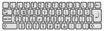
But why don’t most other languages use a similar convention? One factor is typing efficiency: <- requires three keystrokes, while = only requires one (although you eventually get used to it). However, there’s also a historical element here: early keyboards designed for statistical computing actually had a dedicated <- key, which made the operator as convenient as = (source):
y and assign it the value of 5 * 3. Then display the value of y on the console.z that is half of the value of y, and then display the value of z on the console.There are many basic functions in R that you can use. For example, the sqrt() function calculates the square root of a number. I know that it could be annoying to remember all the functions, but luckily we have the powerful AIs to help us. It is pretty easy to use Copilot, a powerful AI tool developed by Github, to get the function you need. It is straightforward to use it in RStudio (link).
We will discuss the use of agent AI towards the end of the course.
However, AIs can be unreliable sometimes. We will discuss unit testing towards the end of the course. As a first step, you can always use the ? to double check when you are unsure about the function. For example, to see the documentation R has on the sqrt() function, you can use the following code:
In addition, you should check some simple cases to make sure the function works as expected. For example, you can use the following code to check the sqrt() function:
sqrt(1) == 1[1] TRUEsqrt(4) == 2[1] TRUETo unlock R’s full potential, you’ll often need to install additional packages—think of them as apps that extend your smartphone’s capabilities. This is a one-time process for each package on your computer. For example, to install the ggplot2 package:
install.packages("ggplot2")After that, simply load it when you need it:
library(ggplot2)This is the first design inconsistencies when using R: when installing a package, you enclose its name in quotes, but when loading it, you don’t. It’s a small quirk, but one that can trip you up if you’re not careful (speaking from experience :-(
There will be many others along the way. I will try to point them out as we go along.
Not all packages are on CRAN. Many are on GitHub, GitLab, or other platforms. The pak package provides a universal way to install packages from any source. For CRAN packages:
# install.packages("pak")
pak::pak("ggplot2")pak first (one-time setup).
You can also install multiple packages at once:
pak::pak(c("ggplot2", "dplyr", "palmerpenguins"))And install packages from GitHub:
pak::pak("cttobin/ggthemr")ggthemr package directly from GitHub.
What is this mysterious :: here? It simply means that we are loading the pak() function from the pak package. It allows you to access a function from a package without loading the entire package. This can help avoid conflicts with other packages that might have a similarly named function (which is a huge source for hidden errors!).
I highly recommend this approach, because pak automatically detects whether a package is already installed (and skips it if so), clearly documents which dependencies it comes with, and it provides a universal way to install packages from different sources. We will use pak throughout this course.
Install the package gt using the standard method and the pak method.
As stated in its official website:
The tidyverse is an opinionated collection of R packages designed for data science. All packages share an underlying design philosophy, grammar, and data structures.
Installing it may take a bit:
install.packages("tidyverse")Once done, loading it is straightforward and a common part of most R scripts (I usually begin nearly all my scripts with this line):
library(tidyverse)Warning: package 'tibble' was built under R version 4.4.3Warning: package 'dplyr' was built under R version 4.4.3Warning: package 'lubridate' was built under R version 4.4.3── Attaching core tidyverse packages ──────────────────────── tidyverse 2.0.0 ──
✔ dplyr 1.2.0 ✔ readr 2.1.5
✔ forcats 1.0.0 ✔ stringr 1.6.0
✔ lubridate 1.9.5 ✔ tibble 3.3.1
✔ purrr 1.2.0.9000 ✔ tidyr 1.3.1
── Conflicts ────────────────────────────────────────── tidyverse_conflicts() ──
✖ dplyr::filter() masks stats::filter()
✖ dplyr::lag() masks stats::lag()
ℹ Use the conflicted package (<http://conflicted.r-lib.org/>) to force all conflicts to become errorsAs you can see, Looking at the message generated by executing the above line, we see that nine packages are now loaded. They are called ggplot2, tibble, and so on. We will get to know these in more detail throughout the class.
As you can see from the message, it shows what conflicts are there. The two conflicts are horrible design choices in tidyverse. Many mysterious bugs happen because of these conflicts. To avoid these, you can use the following code:
library(conflicted)
library(tidyverse)
conflict_prefer("filter", "dplyr")
conflict_prefer("lag", "dplyr")conflicted package.
tidyverse package.
filter, always prefer dplyr.
lag, always prefer dplyr.
Another way is to just write your code using the package::funcion() format:
dplyr::filter()
dplyr::lag()
Given how often you’ll use these functions, I find it annoying with this approach. But it’s a personal choice.
If you do not want to see the messages (although I do not recommend), you can use the suppressPackageStartupMessages() function. For example, you can use the following code to load the tidyverse package:
suppressPackageStartupMessages(library(tidyverse))This approach hides the typical start-up output, though it remains entirely optional.
We’ll rely on the tidyverse extensively throughout this course.