12  Visualizing Distribution

Class Objectives:

1. Distribution of a single variable
2. Distribution of multiple variables
3. Distribution of a variable across multiple groups

Packages for this chapter

If you haven’t installed the following packages, run this code:

pak::pak(c("tidyverse", "janitor", "palmerpenguins", "gghighlight", "ggridges", "patchwork", "geomtextpath", "ggdensity", "ggbeeswarm", "ggforce", "gghalves", "ggalt"))

Data distributions are central to data analysis. We’ll explore several methods for visualizing distributions in R using ggplot2 and related packages.

Load tidyverse and palmerpenguins so we can use functions such as ggplot() and the penguins dataset directly. For other packages, use package::function(), such as janitor::clean_names(), to show where each function comes from. Let us begin by loading these packages and setting the theme.

library(tidyverse)
library(palmerpenguins)
theme_set(theme_minimal())

1

Set all plots to use theme_minimal().

12.1 Single Variable

12.1.1 Histograms

Histograms are a common way to visualize the distribution of a single variable. In this example, we plot the distribution of flipper_length_mm from the penguins dataset:

penguins |>
    ggplot(aes(x = flipper_length_mm)) +
    geom_histogram(color = "white")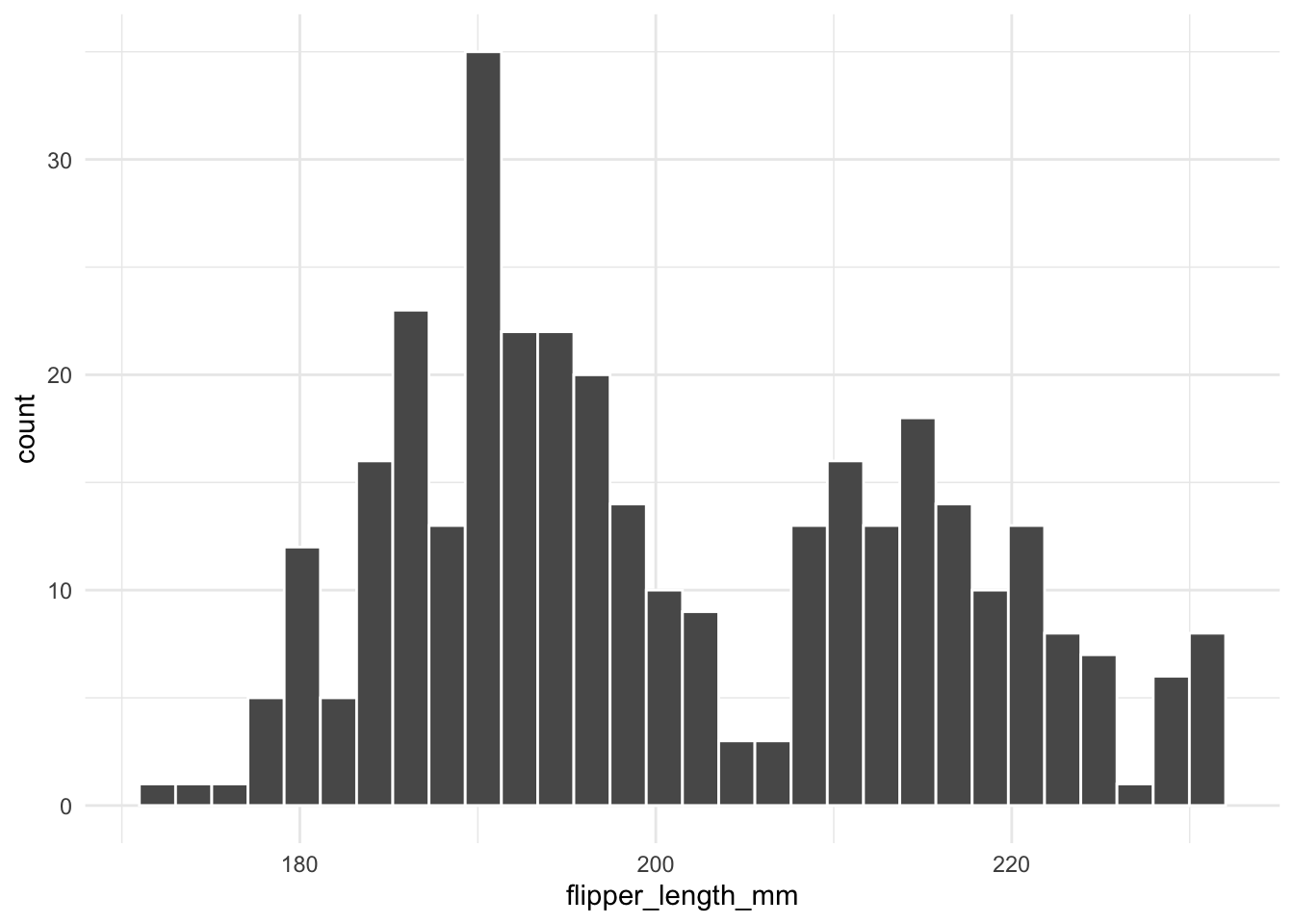

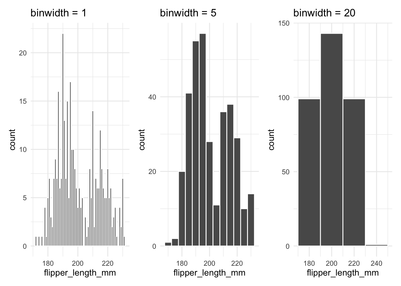
A frequent mistake is to call geom_histogram() without specifying the binwidth. When you don’t set it, ggplot2 uses bins = 30 (and prints a message asking you to pick a better value), which may not reveal important details in your data. The example below shows how changing the bin width affects the histogram:

c(1, 5, 20) |>
    map(\(w) penguins |>
        ggplot(aes(x = flipper_length_mm)) +
        geom_histogram(binwidth = w, color = "white") +
        labs(title = paste("binwidth =", w))
    ) |>
    patchwork::wrap_plots()

1

binwidth sets the width of each bin in the units of the x variable (here millimetres).

12.1.2 Density Plots

Density plots provide a smooth estimate of the distribution. For example, the following code creates a density plot for flipper_length_mm:

Basic density plot

It is very easy to draw a density plot.

penguins |>
    ggplot(aes(x = flipper_length_mm)) +
    geom_density()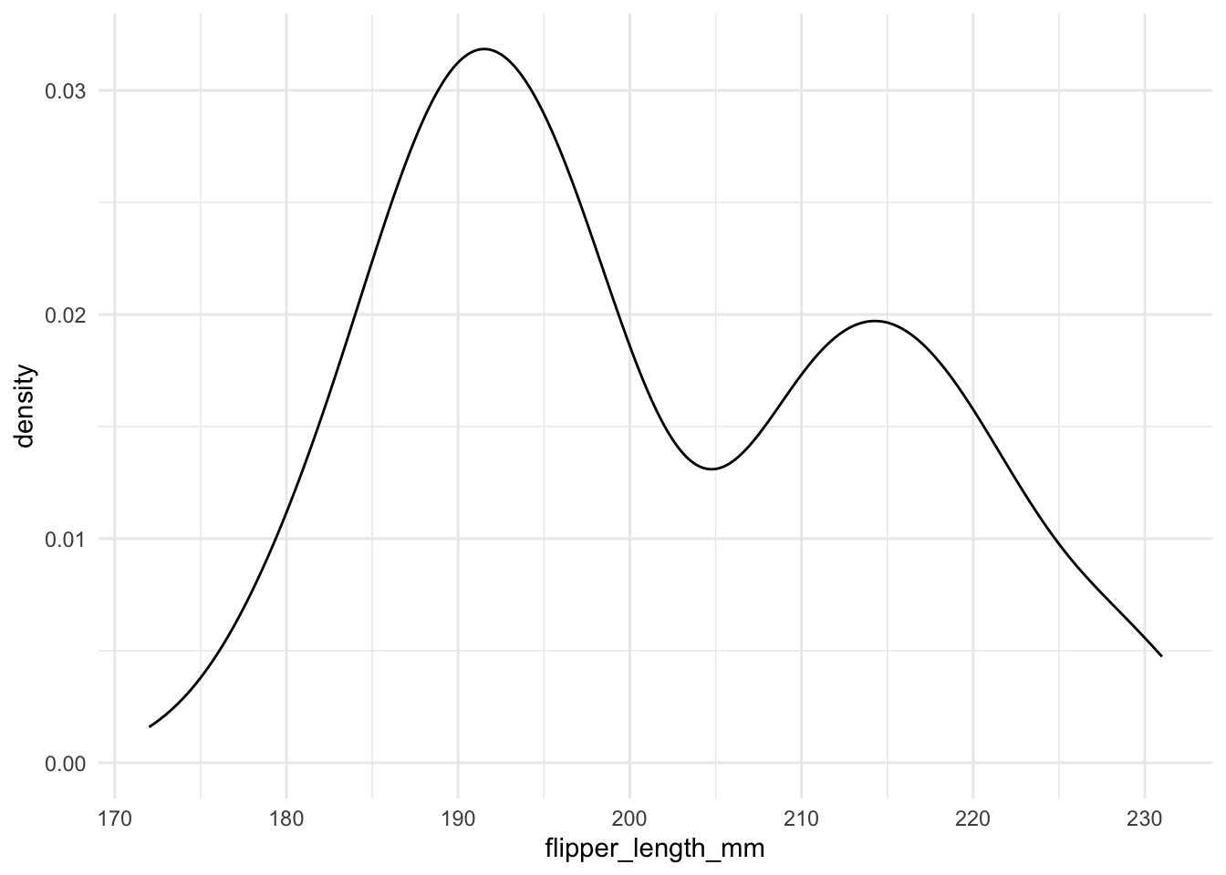

Filled density plot

An unfilled outline is often harder to read than a filled shape, so it is usually better to fill the area under the curve (geom_density() with fill = "what color you like").

penguins |>
    ggplot(aes(x = flipper_length_mm)) +
    geom_density(fill = "lightblue")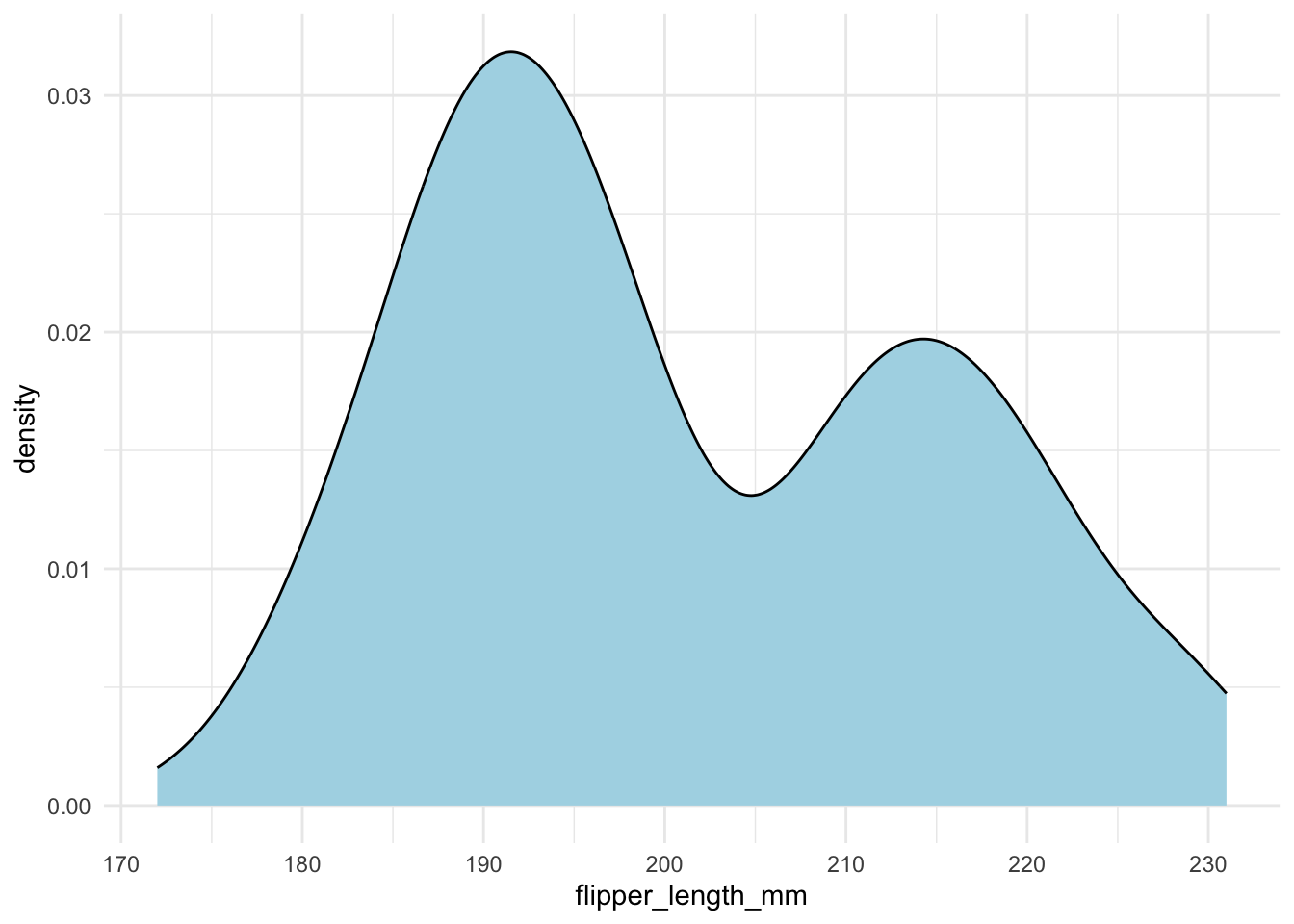

Show the actual data points

It is also a good idea to show the actual data points. You can use geom_rug() to do this.

penguins |>
    ggplot(aes(x = flipper_length_mm)) +
    geom_density(fill = "lightblue") +
    geom_rug()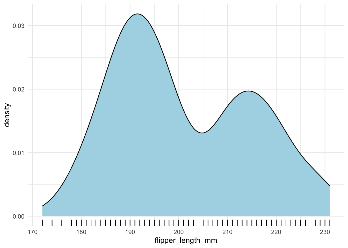

However, when you have a lot of data points, it is better to use geom_hdr_rug() from the ggdensity package.

penguins |>
    ggplot(aes(x = flipper_length_mm)) +
    geom_density(fill = "lightblue") +
    ggdensity::geom_hdr_rug()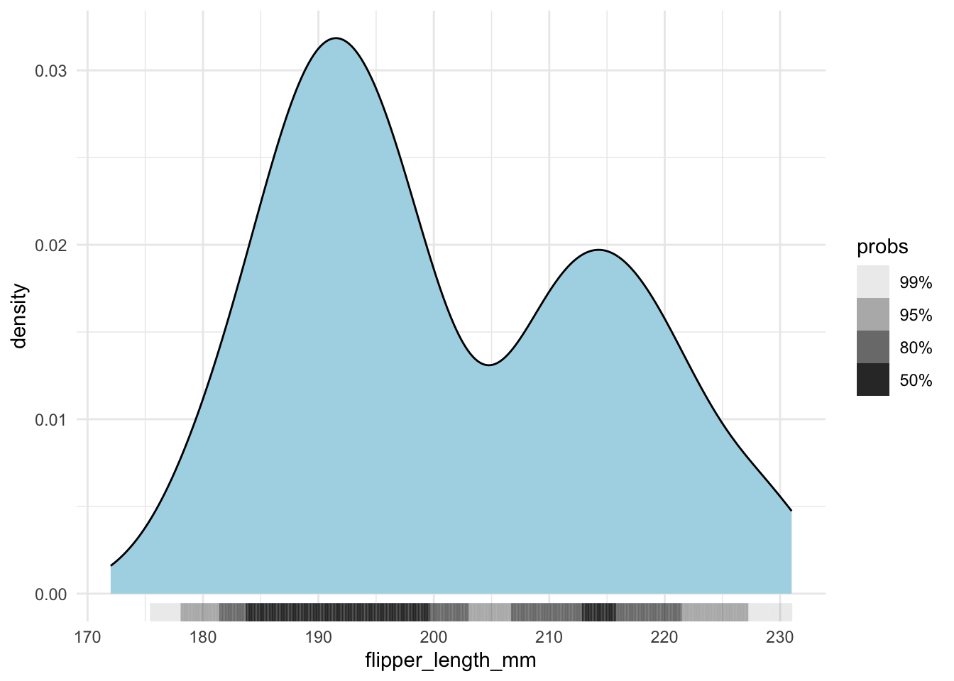

A common pitfall is that the density curve may extend beyond the actual data range. To illustrate, if you normalize your data to range from 0 to 1, the density estimate might still spill outside these bounds. Consider the following example where we normalize the flipper lengths and then set explicit x-axis limits (with xlim(), points outside the limits are dropped, which is why we suppress warnings here):

penguins |>
    drop_na(flipper_length_mm) |>
    mutate(flipper_length_mm_normalized = (flipper_length_mm - min(flipper_length_mm)) / (max(flipper_length_mm) - min(flipper_length_mm))) |>
    ggplot(aes(x = flipper_length_mm_normalized)) +
    geom_density(fill = "lightblue") +
    xlim(-.2, 1.2)

1

We set the x-axis limits to [-0.2, 1.2] to illustrate the issue.

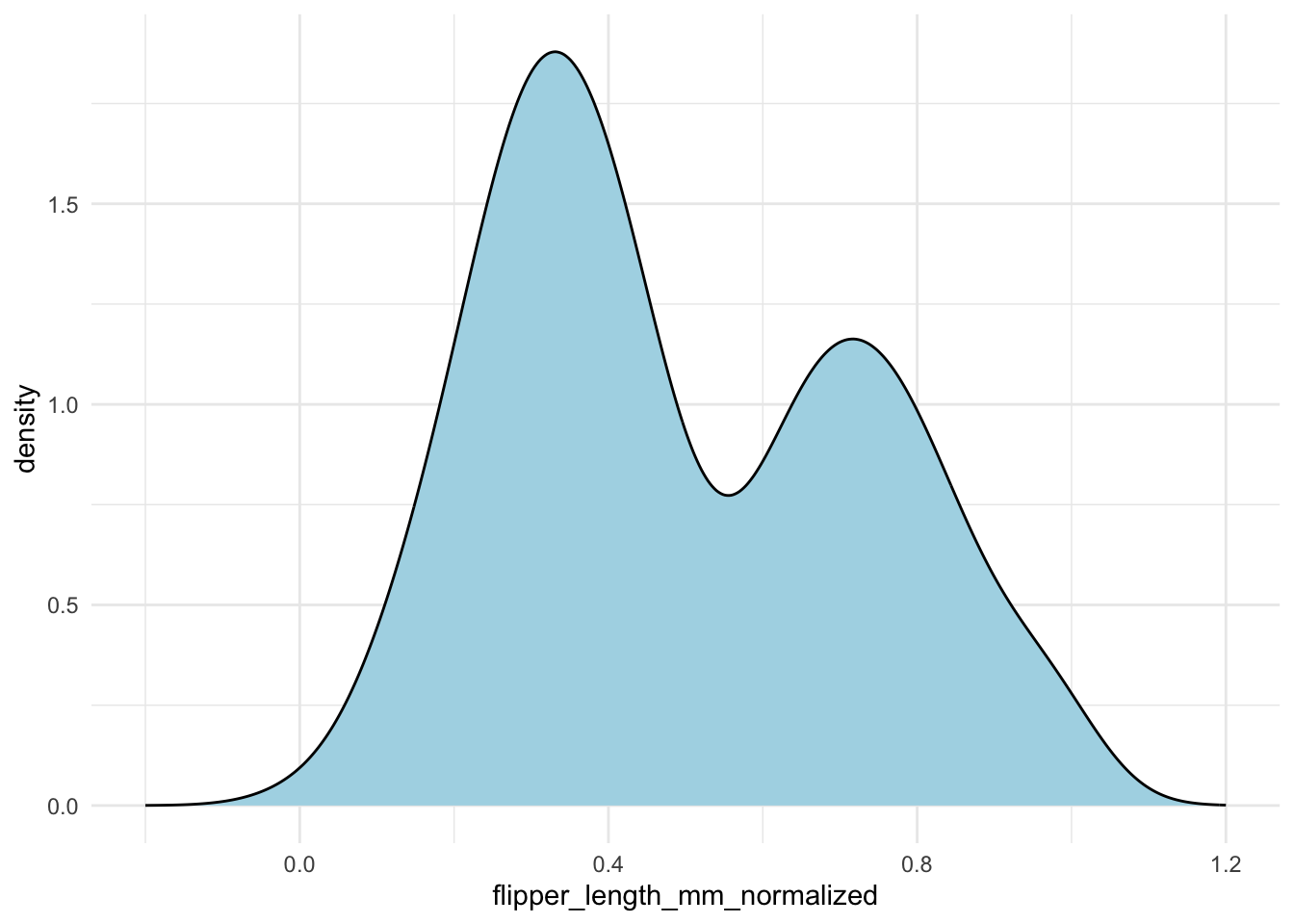
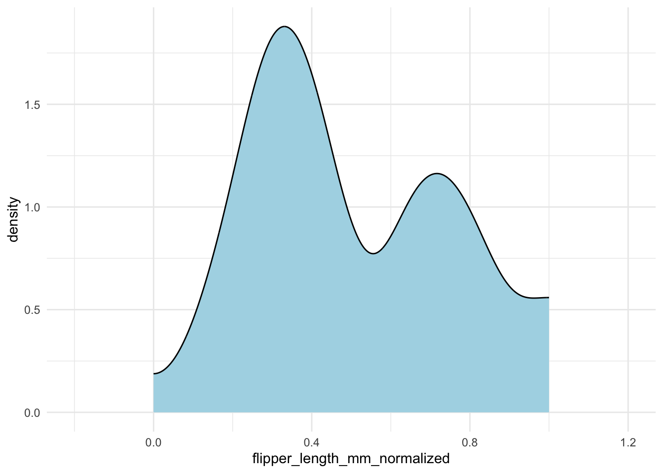
Without careful inspection, you might not notice that the density extends outside the [0, 1] interval. To fix this, you can specify the bounds in geom_density():

penguins |>
    drop_na(flipper_length_mm) |>
    mutate(flipper_length_mm_normalized = (flipper_length_mm - min(flipper_length_mm)) / (max(flipper_length_mm) - min(flipper_length_mm))) |>
    ggplot(aes(x = flipper_length_mm_normalized)) +
    geom_density(fill = "lightblue",
                bounds = c(0, 1)) +
    xlim(-.2, 1.2)

1

We specify the bounds in geom_density() to ensure the density curve stays within the [0, 1] interval.

Alternative density estimate

The ggalt package’s geom_bkde() function offers a binned kernel density estimate that can be faster on large data.

12.2 Comparing More Than One Variable

12.2.1 Histograms vs Density

As a general rule, DON’T use Histograms naively when dealing with multiple variables. For example, all three examples below are difficult to efficiently compare the distribution of flipper length across different species.

Overlapping histograms

Each group is plotted in the same space with transparency:

penguins |>
    ggplot(aes(x = flipper_length_mm, group = species, fill = species)) +
    geom_histogram(color = "white", alpha = .5,position = "identity") +
    theme(legend.position = "top")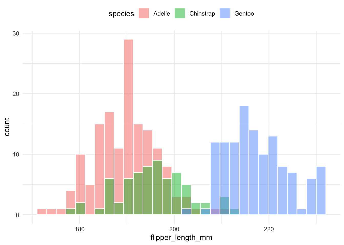

Stacked Histograms

Histograms are stacked on top of each other to compare proportions:

penguins |>
    ggplot(aes(x = flipper_length_mm, group = species, fill = species)) +
    geom_histogram(color = "white", position = "stack") +
    theme(legend.position = "top")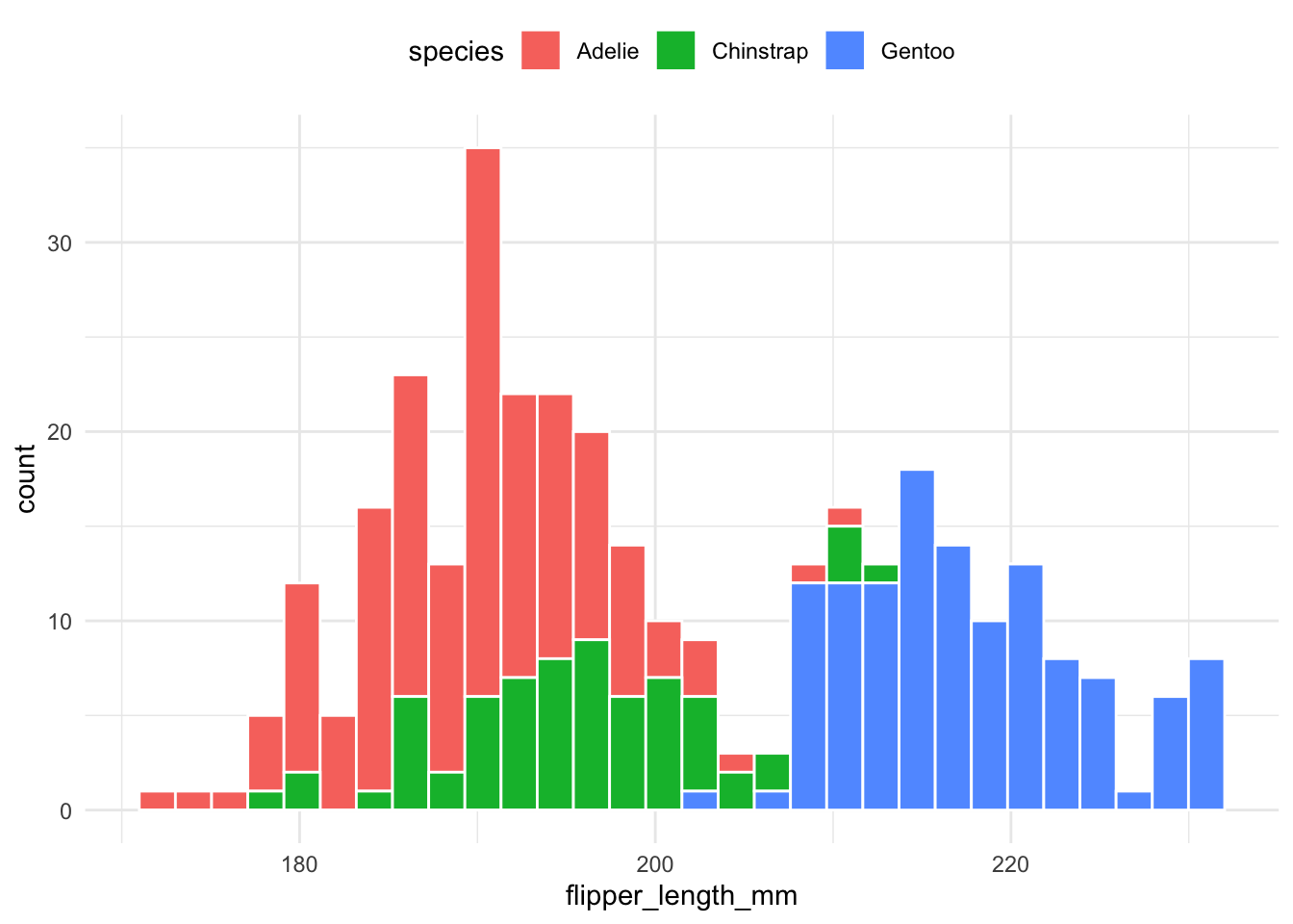

Side by side histograms

Histograms for each group are placed next to one another for easier comparison:

penguins |>
    ggplot(aes(x = flipper_length_mm, group = species, fill = species)) +
    geom_histogram(color = "white", position = "dodge") +
    theme(legend.position = "top")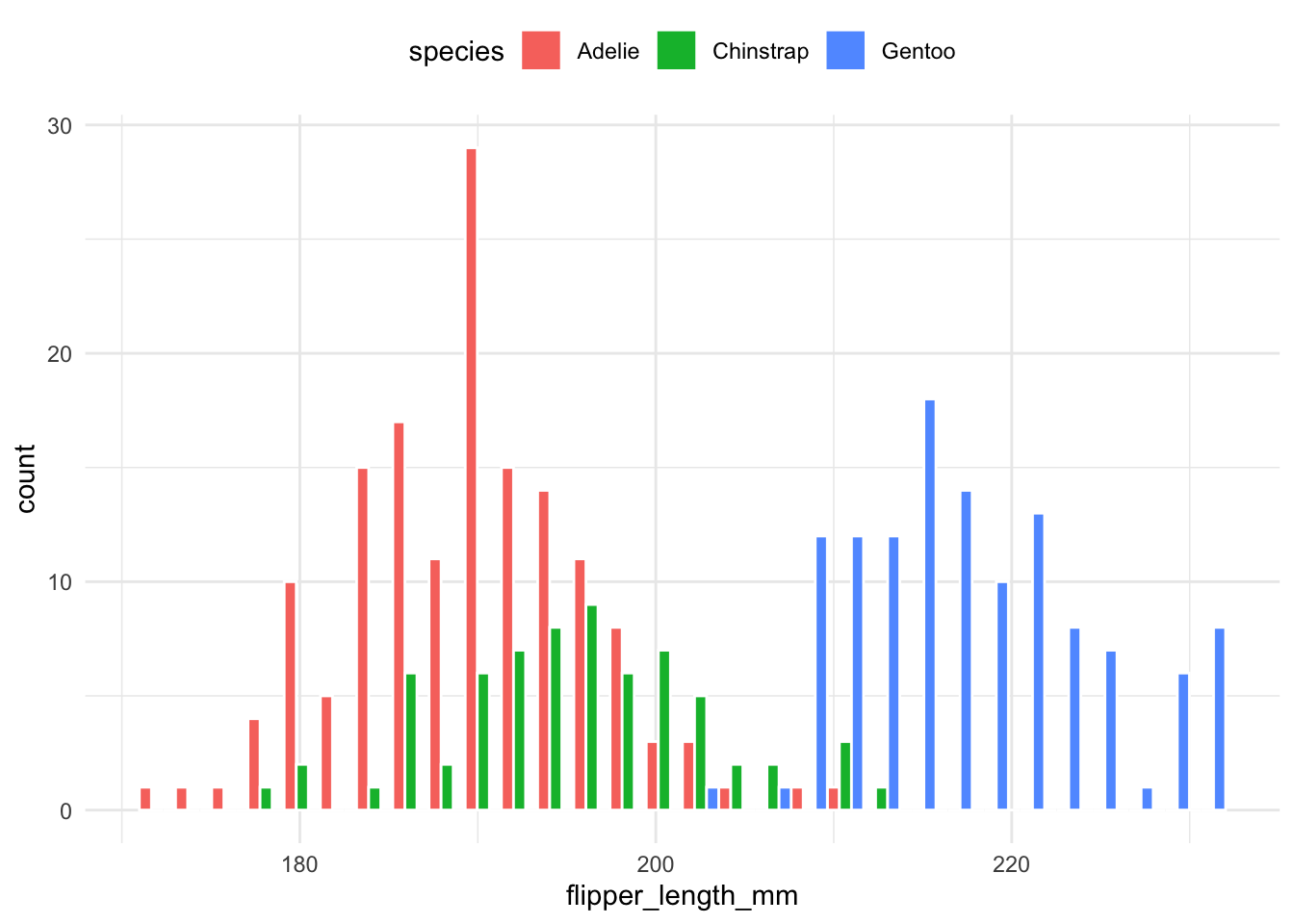

Density plots are generally easier to compare when multiple groups are involved. The following code overlays density curves for each species:

penguins |>
    ggplot(aes(
        x = flipper_length_mm,
        group = species,
        fill = species,
        color = species)) +
    geom_density(alpha = .5) +
    theme(legend.position = "top")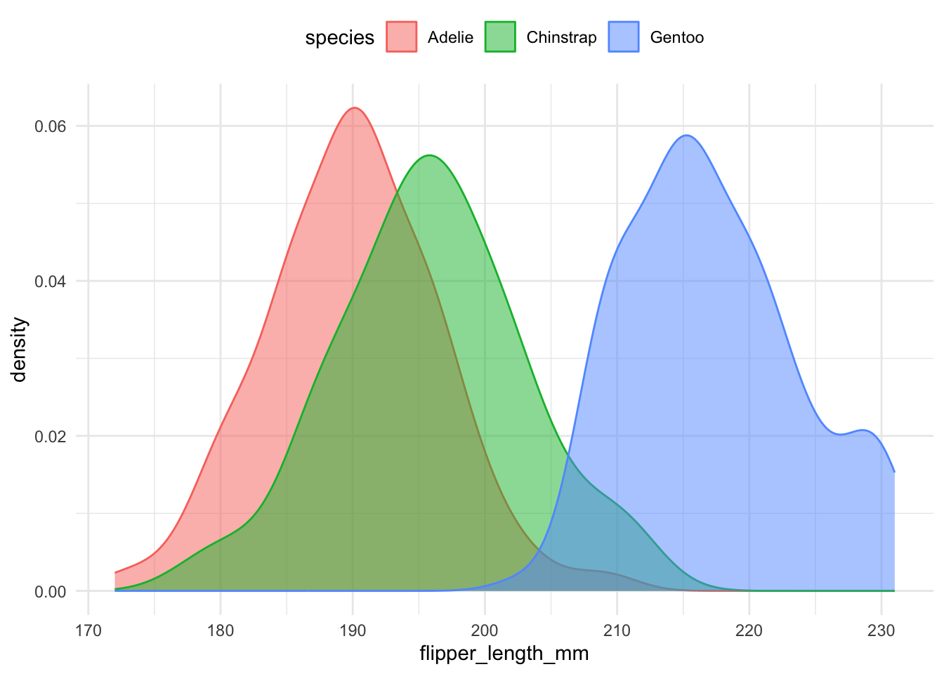

Legends force the reader to look back and forth between the plot and the key, so direct labelling is often better. The package geomtextpath provides a way to add text to the density plot.

penguins |>
    ggplot(aes(x = flipper_length_mm, group = species, color = species)) +
    geomtextpath::geom_textdensity(aes(label = species), size = 5) +
    theme(legend.position = "none")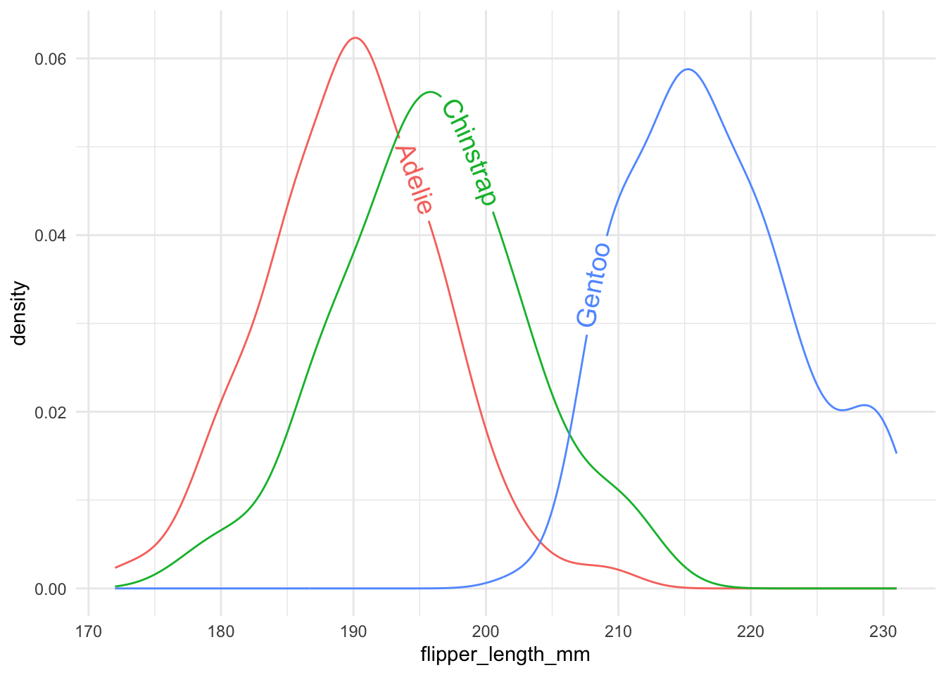

12.2.2 Better Variations for Group Comparisons

There are many variations of density/histogram plots that are more informative and aesthetically pleasing. I particularly like two of them.

Separated plots

The most simple way is to just plot each group in a separate plot.

penguins |>
    ggplot(aes(x = flipper_length_mm,
               fill = species)) +
    geom_histogram(color = "white") +
    facet_wrap(~species)

1

create a separate plot for each species.

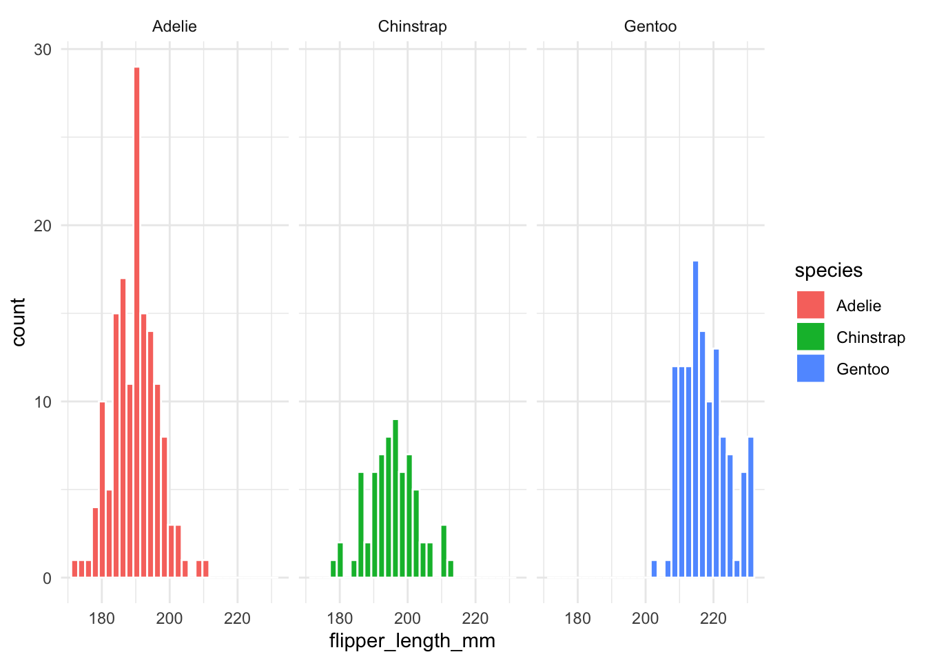
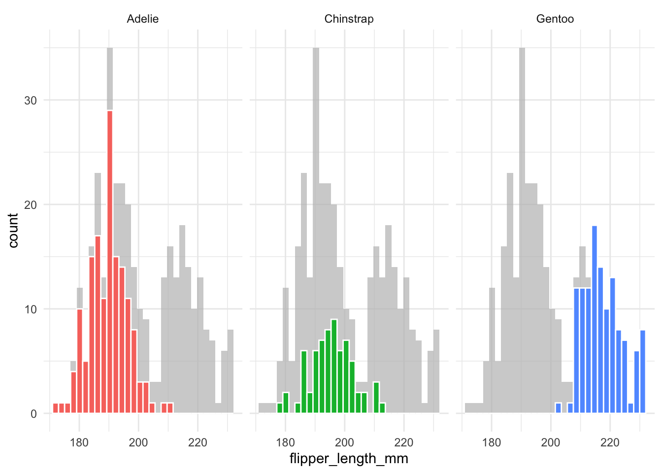
However, this is not very informative as it lacks the information about how one group compares to the others. To solve this, faceting and highlighting each group can be very effective. We can easily do this with the gghighlight package:

penguins |>
    ggplot(aes(x = flipper_length_mm,
               fill = species)) +
    geom_histogram(color = "white") +
    gghighlight::gghighlight() +
    facet_wrap(~species)

1

gghighlight() is used to highlight the data points for each species.

2

facet_wrap(~species) is used to create a separate plot for each species.

The same idea works for density plots. Note that each species’ density is scaled so that the area under its curve is 1, so the heights show the shape of each distribution but not how many penguins each species has. If you want the heights to reflect group sizes, map y = after_stat(count) instead.

penguins |>
    ggplot(aes(x = flipper_length_mm,
               fill = species)) +
    geom_density(color = NA) +
    gghighlight::gghighlight(unhighlighted_params = list(fill = "grey85")) +
    facet_wrap(~species)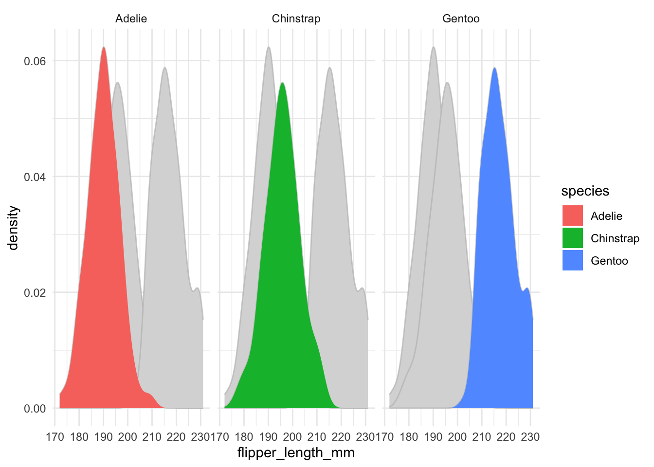

Mirror density

When comparing two groups, a mirror density plot places one density curve above and one below the horizontal axis. This example compares male and female penguins:

penguins |>
    ggplot(aes(x = flipper_length_mm)) +
    geom_density(
        data = filter(penguins, sex == "male"),
        aes(y = after_stat(density)),
        alpha = .5, fill = "#69b3a2", color = "black") +
    geom_label( aes(x=180, y=0.02, label="male"), color="#69b3a2", size = 5) +
    geom_density(
        data = filter(penguins, sex == "female"),
        aes(y = -after_stat(density)),
        alpha = .5, fill = "#404080", color = "black") +
    geom_label( aes(x=228, y=-0.01, label="female"), color="#404080", size = 5)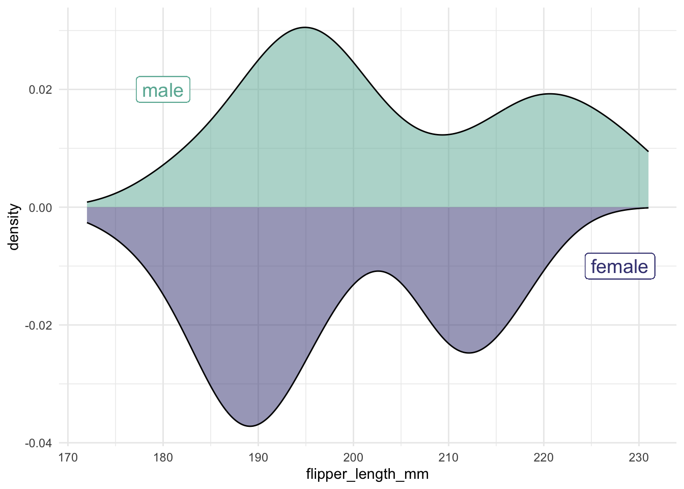

12.3 Many distributions at once

Sometimes, you need to display distributions for many groups simultaneously. For example, we use the lincoln_weather dataset (from the ggridges package) to demonstrate different approaches.

As in the data-import chapter, first use janitor::clean_names() to standardize the column names. This changes CST to cst and Mean Temperature [F] to mean_temperature_f. We then select the relevant columns, parse the date, and extract the month:

lincoln_weather_clean <- ggridges::lincoln_weather |>
    janitor::clean_names() |>
    select(cst, mean_temperature_f) |>
    mutate(
        cst = ymd(cst),
        month = month(cst, label = TRUE)
    )

12.3.1 Summarizing with Points and Error Bars

One approach is to show the mean along with an error bar. Always be explicit about how you compute the error bar!

Central 95% of the data

This shows the mean with the interval that contains the central 95% of the daily observations (the 2.5% and 97.5% quantiles). It describes the spread of the data, not the uncertainty of the mean.

lincoln_weather_clean |>
    group_by(month) |>
    summarise(mean = mean(mean_temperature_f),
              lower = stats::quantile(mean_temperature_f, 0.025),
              upper = stats::quantile(mean_temperature_f, 0.975)) |>
    ggplot(aes(x = month, y = mean, ymin = lower, ymax = upper)) +
    geom_pointrange()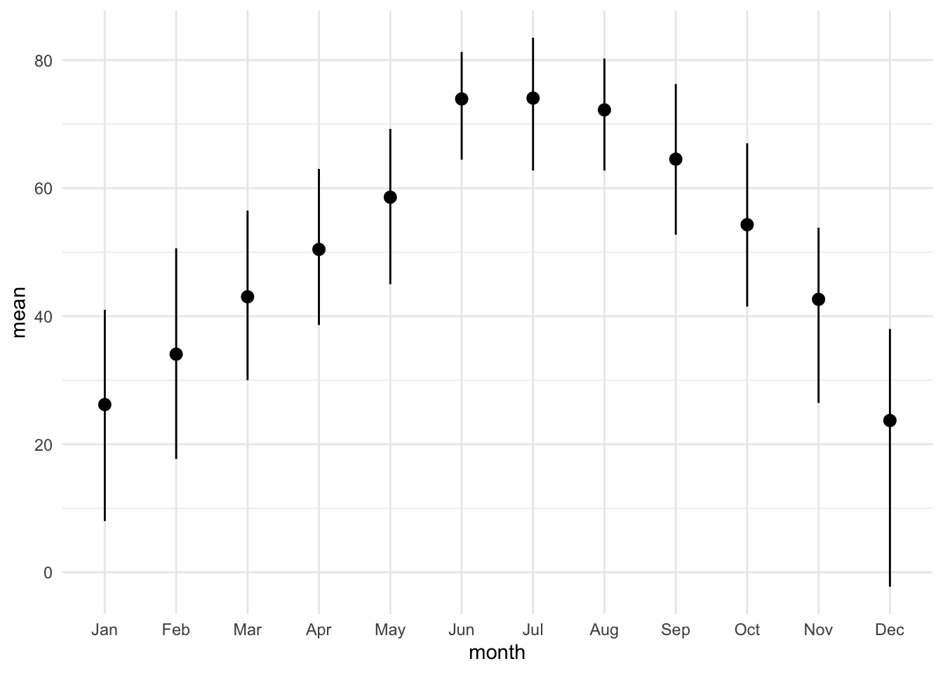

Standard deviation

The standard deviation also describes the spread of the data.

lincoln_weather_clean |>
    group_by(month) |>
    summarise(mean = mean(mean_temperature_f),
              sd = stats::sd(mean_temperature_f)) |>
    ggplot(aes(x = month, y = mean)) +
    geom_pointrange(aes(ymin = mean - sd, ymax = mean + sd))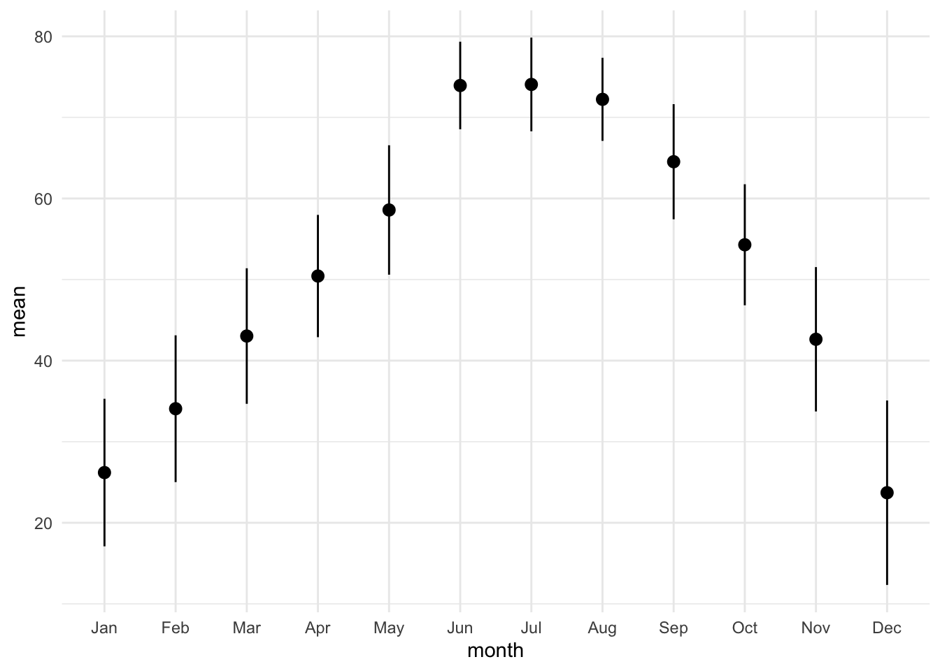

Standard error

The standard error describes the uncertainty of the mean, not the spread of the data.

lincoln_weather_clean |>
    group_by(month) |>
    summarise(mean = mean(mean_temperature_f),
              se = stats::sd(mean_temperature_f) / sqrt(n())) |>
    ggplot(aes(x = month, y = mean)) +
    geom_pointrange(aes(ymin = mean - se, ymax = mean + se))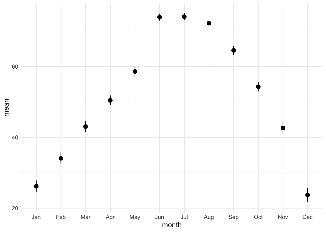

95% confidence interval

A confidence interval for the mean is built from the standard error (a rough approximation that treats the daily values as independent).

lincoln_weather_clean |>
    group_by(month) |>
    summarise(mean = mean(mean_temperature_f),
              se = stats::sd(mean_temperature_f) / sqrt(n()),
              n = n()) |>
    ggplot(aes(x = month, y = mean)) +
    geom_pointrange(aes(ymin = mean - stats::qt(0.975, n - 1) * se,
                        ymax = mean + stats::qt(0.975, n - 1) * se))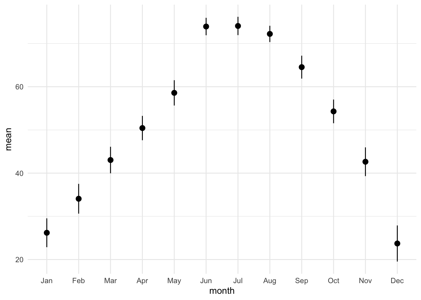

12.3.2 Showing the Full Distribution

Whenever possible, display the full distribution rather than just summary statistics.

Boxplot

lincoln_weather_clean |>
    ggplot(aes(x = month, y = mean_temperature_f)) +
    geom_boxplot()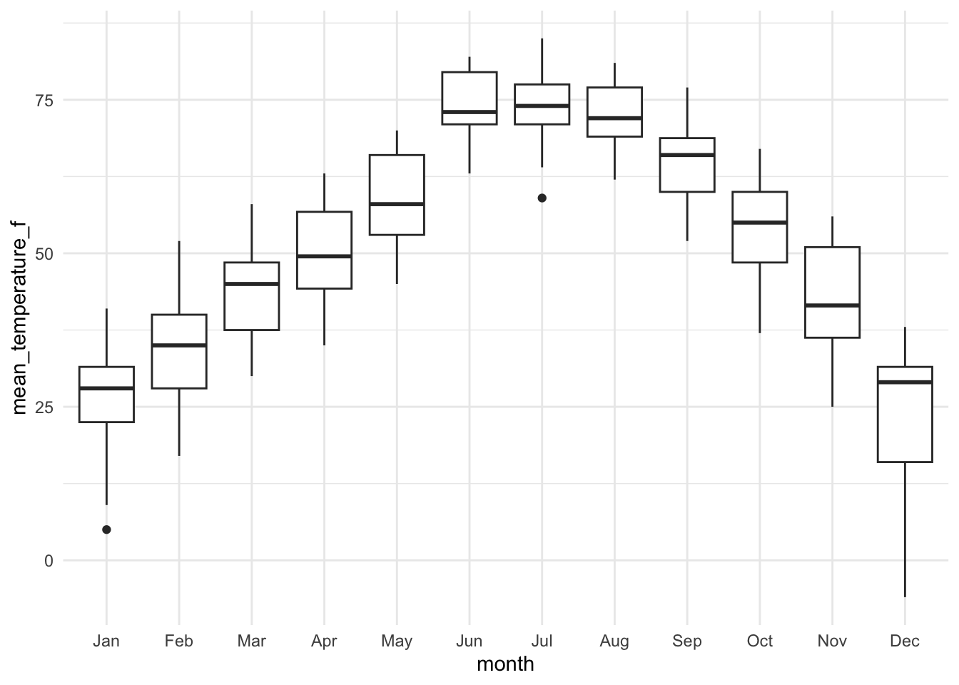

Violin Plot

lincoln_weather_clean |>
    ggplot(aes(x = month, y = mean_temperature_f)) +
    geom_violin()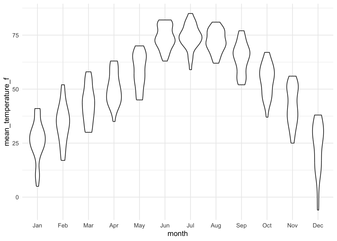

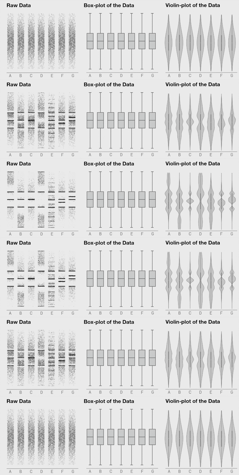
Violin plots (and raw points, see below) can reveal features of the distribution, such as multiple modes, that a boxplot hides. The animated comparison below illustrates this. Keep in mind that a violin drawn from a small sample (each month here has only about 30 observations) is a smoothed estimate and can mislead, which is another reason to show the raw data.

Boxplots versus violin plots on the same data. Source: https://www.research.autodesk.com/publications/same-stats-different-graphs/

12.3.3 Plotting the Actual Data Points

It’s a good idea to show the raw data along with any summaries. This is especially true for real data, where we often have to work with limited samples. It is less useful, or sometimes even advised against, for synthetic data.

DON’t just use geom_point()

lincoln_weather_clean |>
    ggplot(aes(x = month, y = mean_temperature_f)) +
    geom_point(alpha = .5)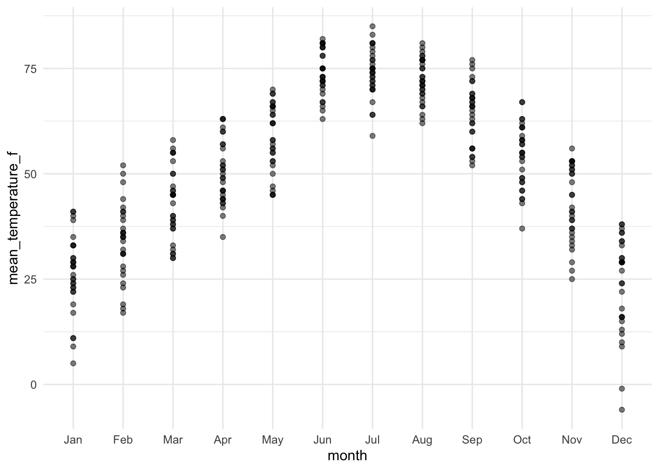

Jittered points

Jittering helps avoid overlapping points:

lincoln_weather_clean |>
    ggplot(aes(x = month, y = mean_temperature_f)) +
    geom_jitter(alpha = .5)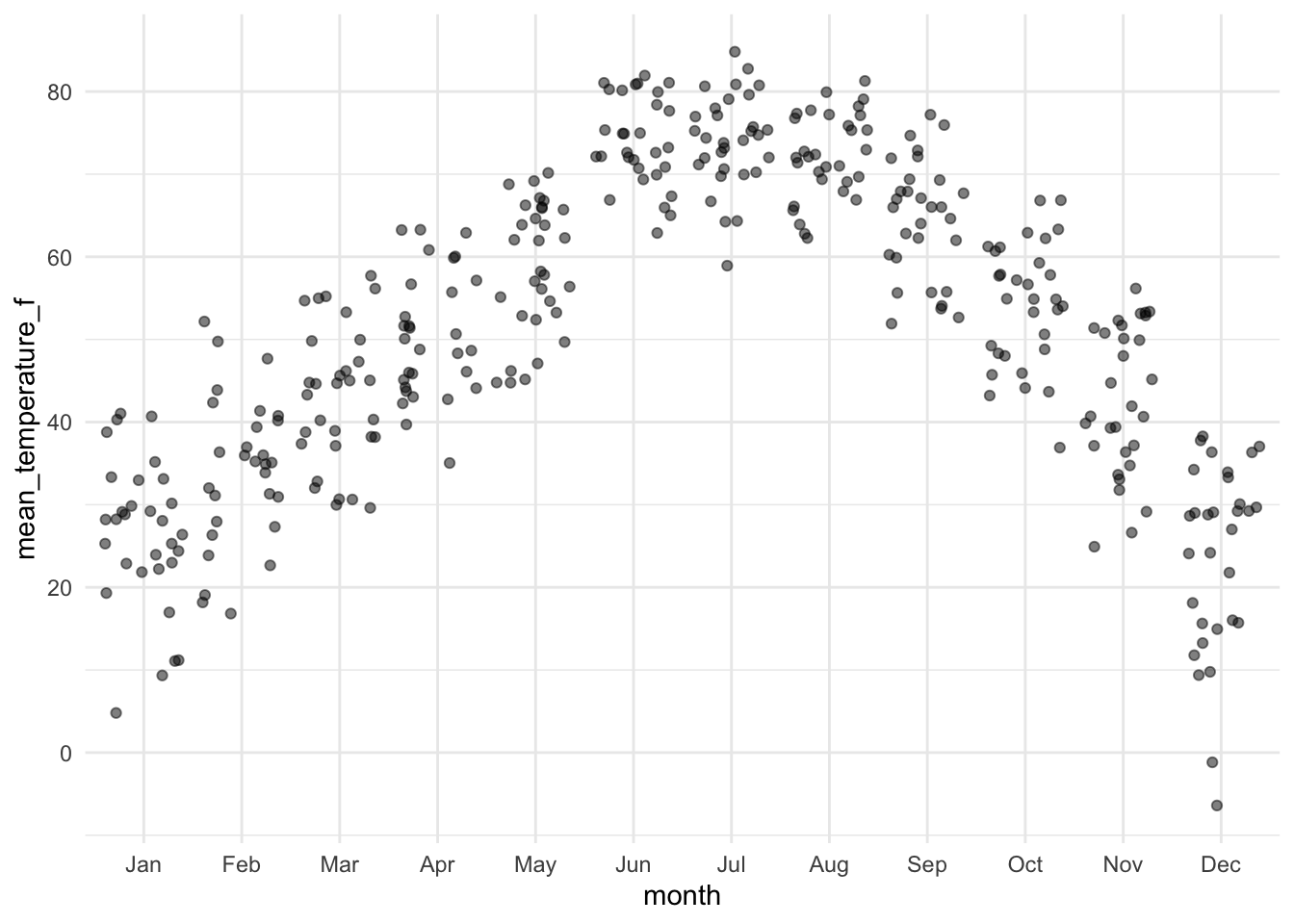

Beeswarm style

For more controlled jittering, use the ggbeeswarm package:

lincoln_weather_clean |>
    ggplot(aes(x = month, y = mean_temperature_f)) +
    ggbeeswarm::geom_quasirandom(varwidth = TRUE)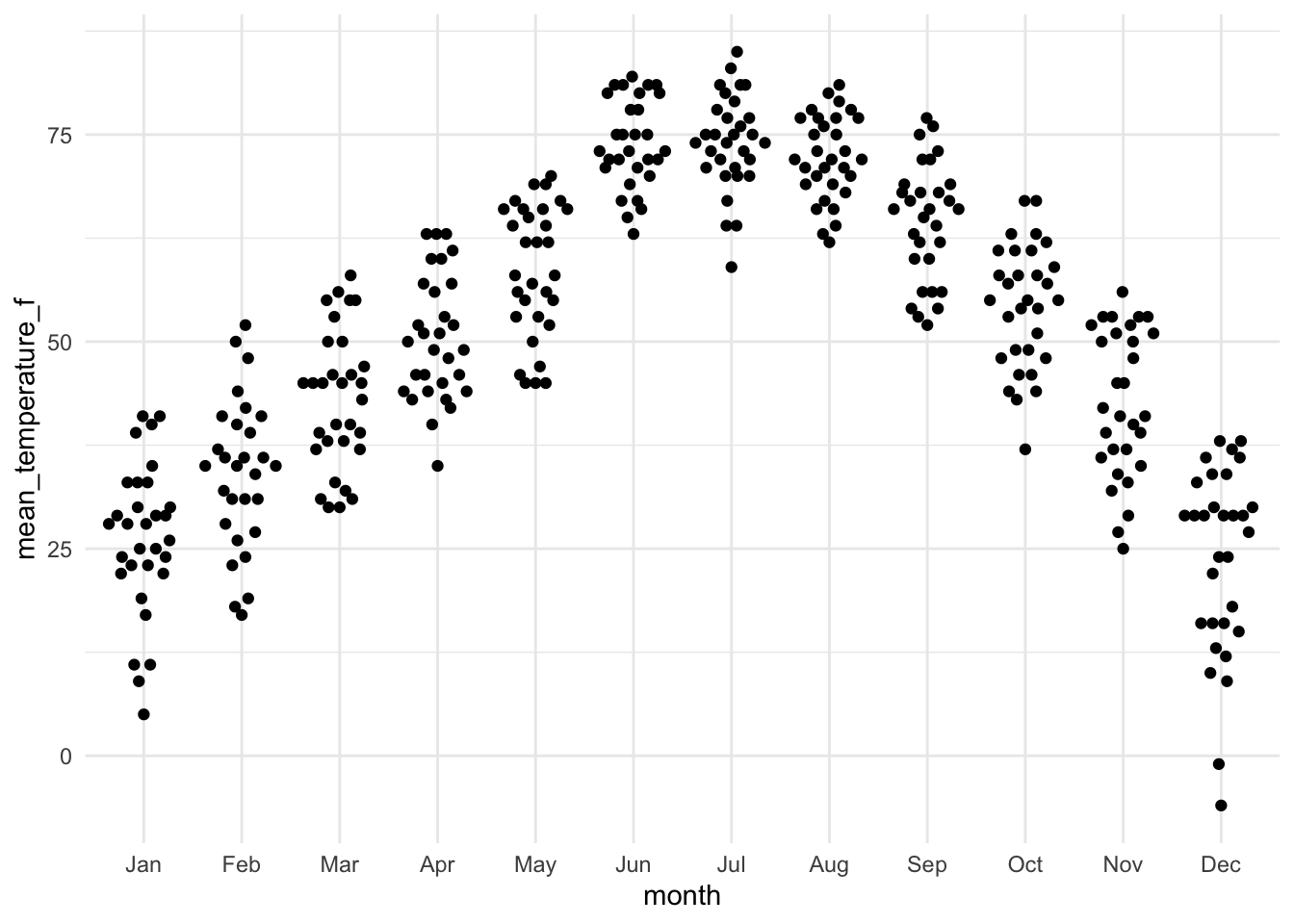

Even better, why not show both the data and the distribution?

Sina plot

lincoln_weather_clean |>
    ggplot(aes(x = month, y = mean_temperature_f)) +
    geom_violin(alpha = .5) +
    ggforce::geom_sina()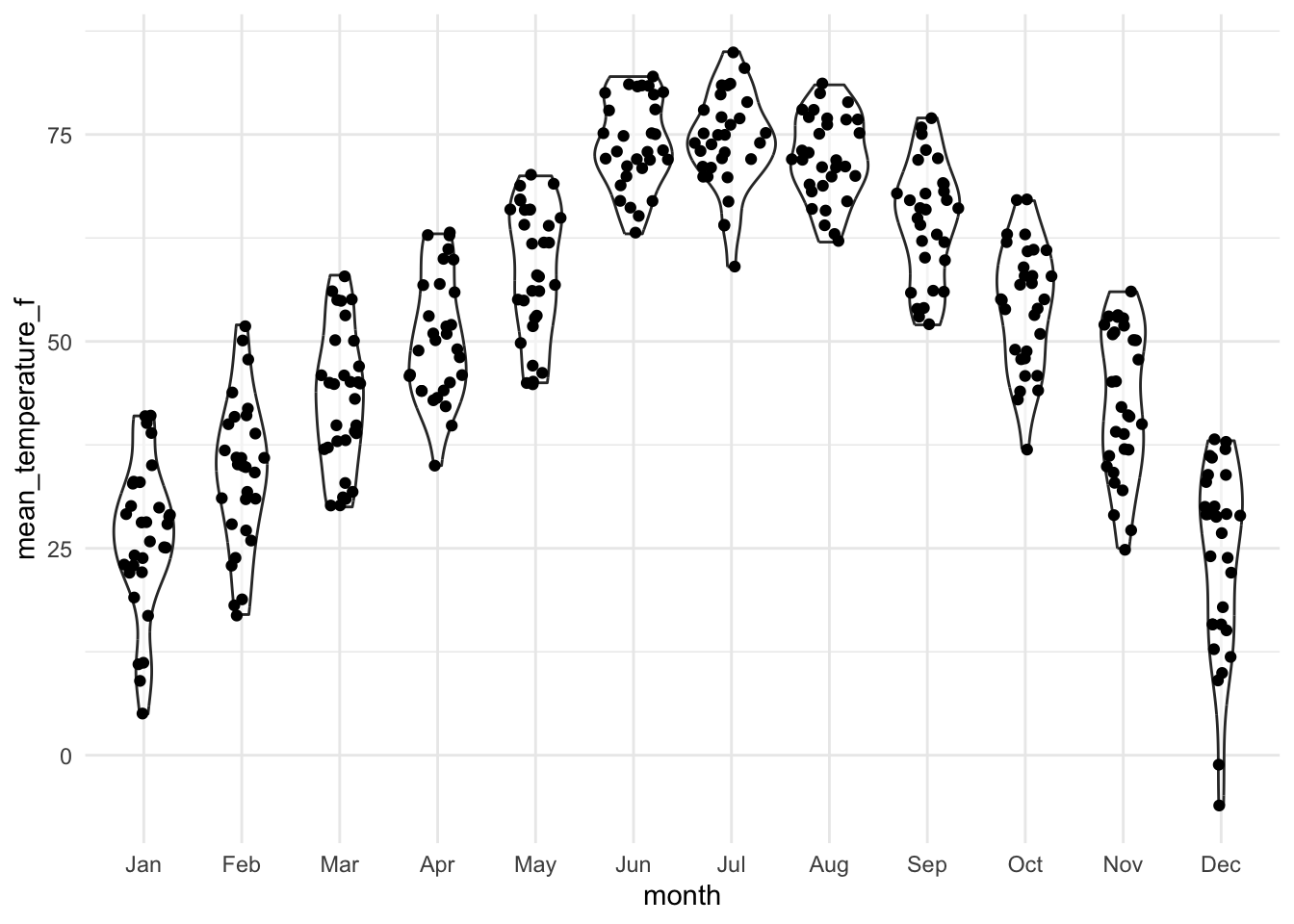

Half-half plot

lincoln_weather_clean |>
    ggplot(aes(x = month, y = mean_temperature_f)) +
    gghalves::geom_half_violin(alpha = .5) +
    gghalves::geom_half_dotplot(method="histodot", stackdir="up", binwidth = 1)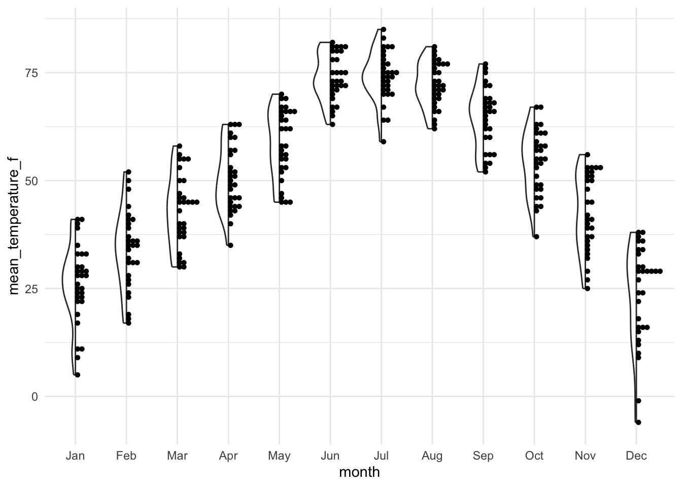

12.3.4 Ridge plot

Ridge plots (also known as joy plots, a name that has since been dropped in favour of “ridgeline plots”) are great for comparing the distribution of a variable across many groups in a compact format. It provides a horizontal axis and a vertical density plot for each group.

lincoln_weather_clean |>
    ggplot(aes(
        x = mean_temperature_f,
        y = month,
        fill = month,
        color = month
    )) +
    ggridges::geom_density_ridges(alpha = .5) +
    ggridges::theme_ridges() +
    theme(legend.position = "none")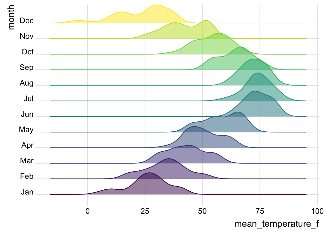

Alternative: Horizon Plots

An issue with ridge plots is that, when the number of groups is large, distributions can be too crowded to be useful. Horizon plots are a great alternative. It uses a very smart trick to avoid overplotting:

How a horizon plot is constructed. Source: https://bernatgel.github.io/karyoploter_tutorial/Tutorial/PlotHorizon/PlotHorizon.html

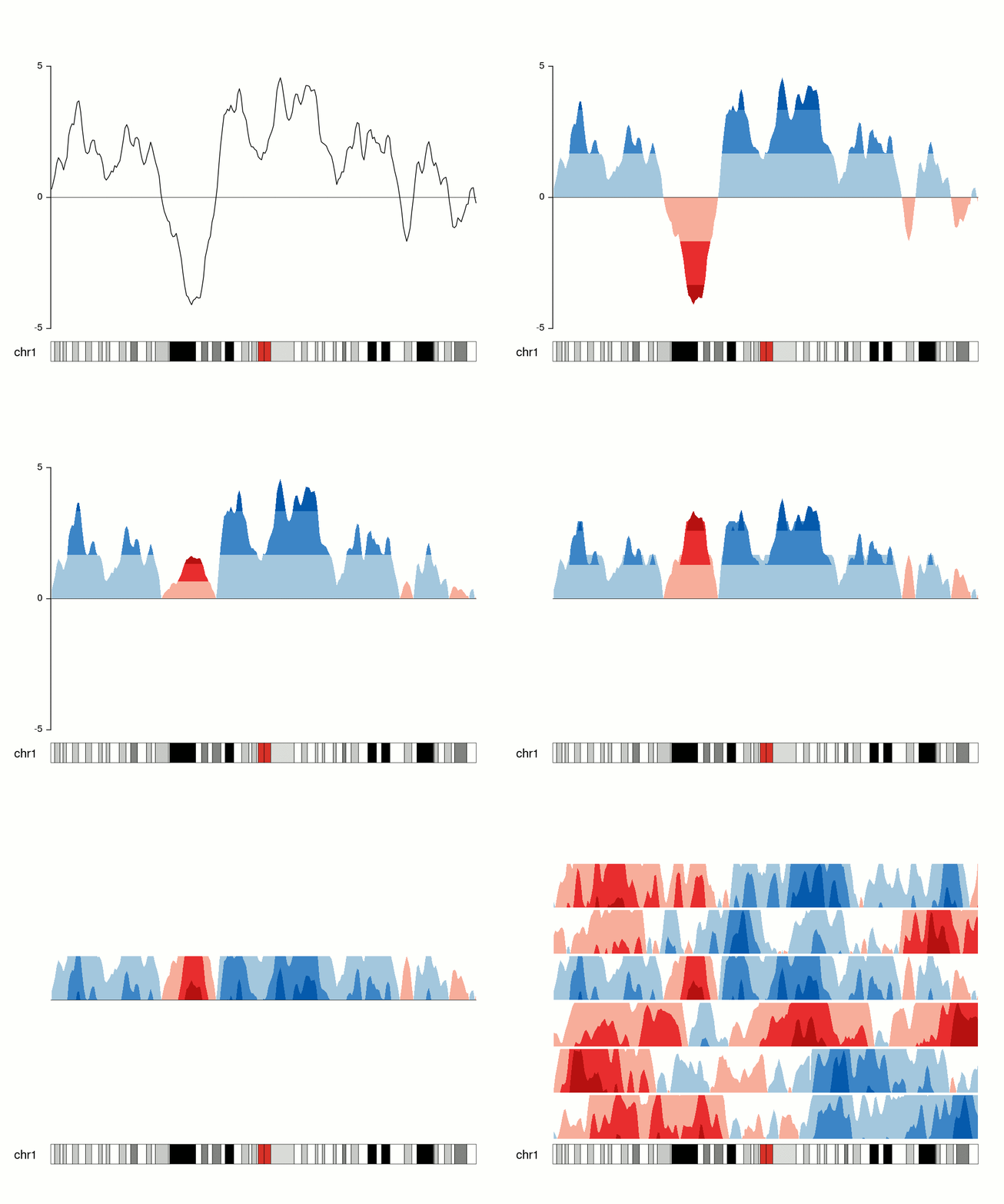
You can use the ggHoriPlot package to create them easily. Check out the documentation here for stunning examples.

However, the risk is that the horizon plot is not a standard plot type that most people are familiar with. Be cautious that other people might have trouble interpreting it.