11 Visualizing Amount

Class Objectives:

Effective use of bar plots
Variations of bar plots
Multiple categories
Treemaps for parts of a whole

Packages for this chapter

If you haven’t installed the following packages, run this code:

pak::pak(c("tidyverse", "palmerpenguins", "MetBrewer", "ggpattern", "ggpol", "waffle", "treemapify", "WeightedTreemaps", "scales", "ggalt", "hrbrthemes", "cttobin/ggthemr"))

Visualizing amounts is a foundational task in data analysis. This tutorial covers best practices, common tools, and key considerations for effective visualizations.

Load tidyverse and palmerpenguins so we can use their functions and the penguins dataset directly. For other packages, use package::function() to show where each function comes from.

library(tidyverse)
library(palmerpenguins)
ggthemr::ggthemr("fresh")

1: This tells R to use the ggthemr package to style all the plots (it is installed from GitHub, see the box above).

ggthemr may print deprecation warnings with recent versions of ggplot2; they come from inside the package and can be ignored.

11.1 Bar plots

Bar plots are among the most straightforward ways to visualize the amount. We have all learnt it very early in school. They’re great when you have discrete categories—like species of penguins—and you want to compare their counts at a glance.

Tha task here is to visualize how many penguins belong to each species in the penguins dataset. Using what we have learned so far, we can do this in a few lines of code:

penguins_count <- penguins |>
    group_by(species) |>
    summarise(n = n()) |>
    ungroup()

1: This tells R to group the data by the species column.
2: This tells R to count the number of rows in each group.
3: This tells R to remove the grouping.

(The same table can be produced in one step with count(species).)

Because we have already counted the penguins, we use geom_col(), which plots the values in y as the bar heights:

penguins_count |> 
    ggplot(aes(x = species, y = n)) +
    geom_col()

1: Uses the ‘n’ column for the bar heights.

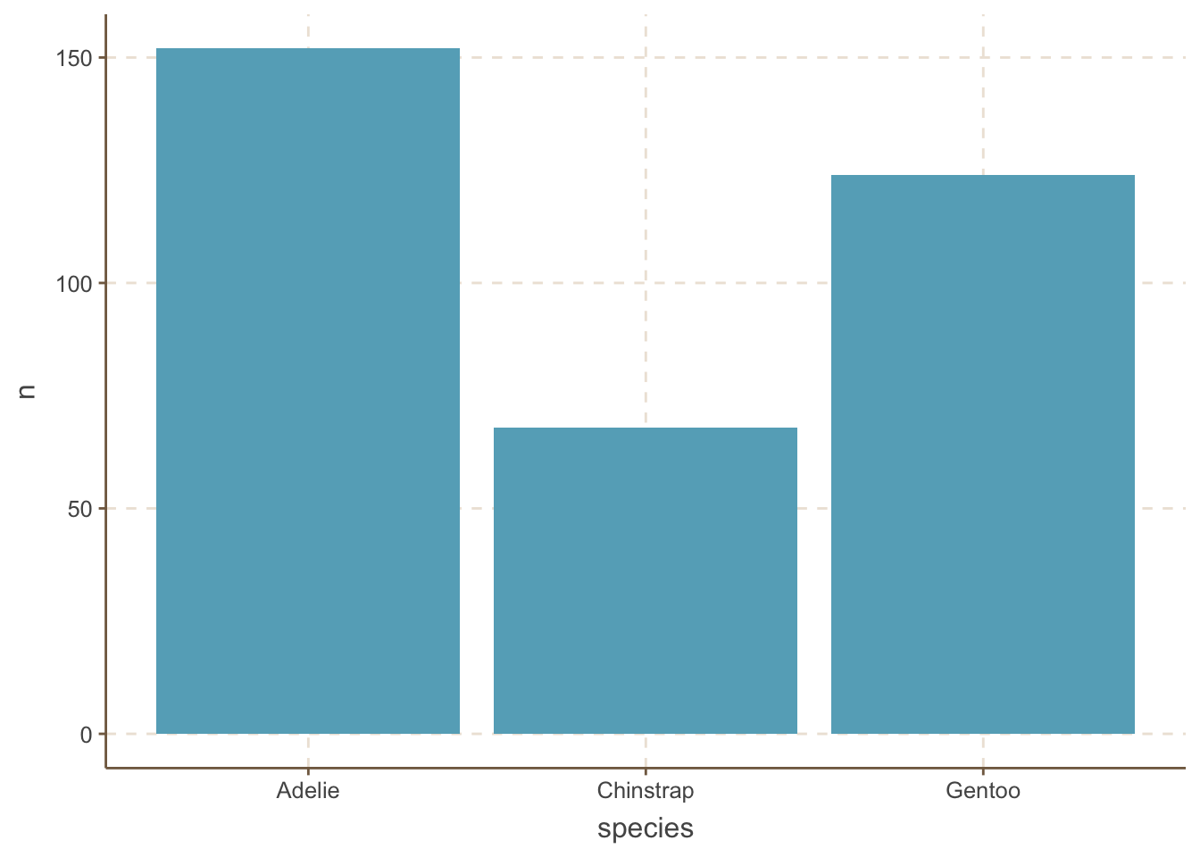
A very common mistake is to use geom_bar() with pre-aggregated data. geom_bar() counts rows by itself (stat = "count"), so if you also map y = n, ggplot2 throws an error (stat_count() must only have an x or y aesthetic). Older code works around this with geom_bar(stat = "identity"), which is exactly what geom_col() does; prefer geom_col(). Alternatively, use geom_bar() on the raw penguins data with no y and let ggplot2 count the rows.

You may think bar plot is so simple. Surprisingly, a study reports that a substantial fraction of biological papers use bar plots in ways that hide the underlying data (for example, bars for small samples of continuous data). Thus, our job is not done yet. Below are a few techniques to make bar plots more informative and visually appealing.

It is useful to add the amount of each category to the bar plot. We can do this by adding a geom_text() layer to the plot.

penguins_count  |> 
    ggplot(aes(x = species, y = n)) +
    geom_col() +
    geom_text(aes(label = n), size = 5,vjust = -0.5) +
    coord_cartesian(clip = 'off')

1: Move the label up by half of the text height (vjust is relative to the label, not in data units).
2: Allow the text to be displayed outside the plot area.

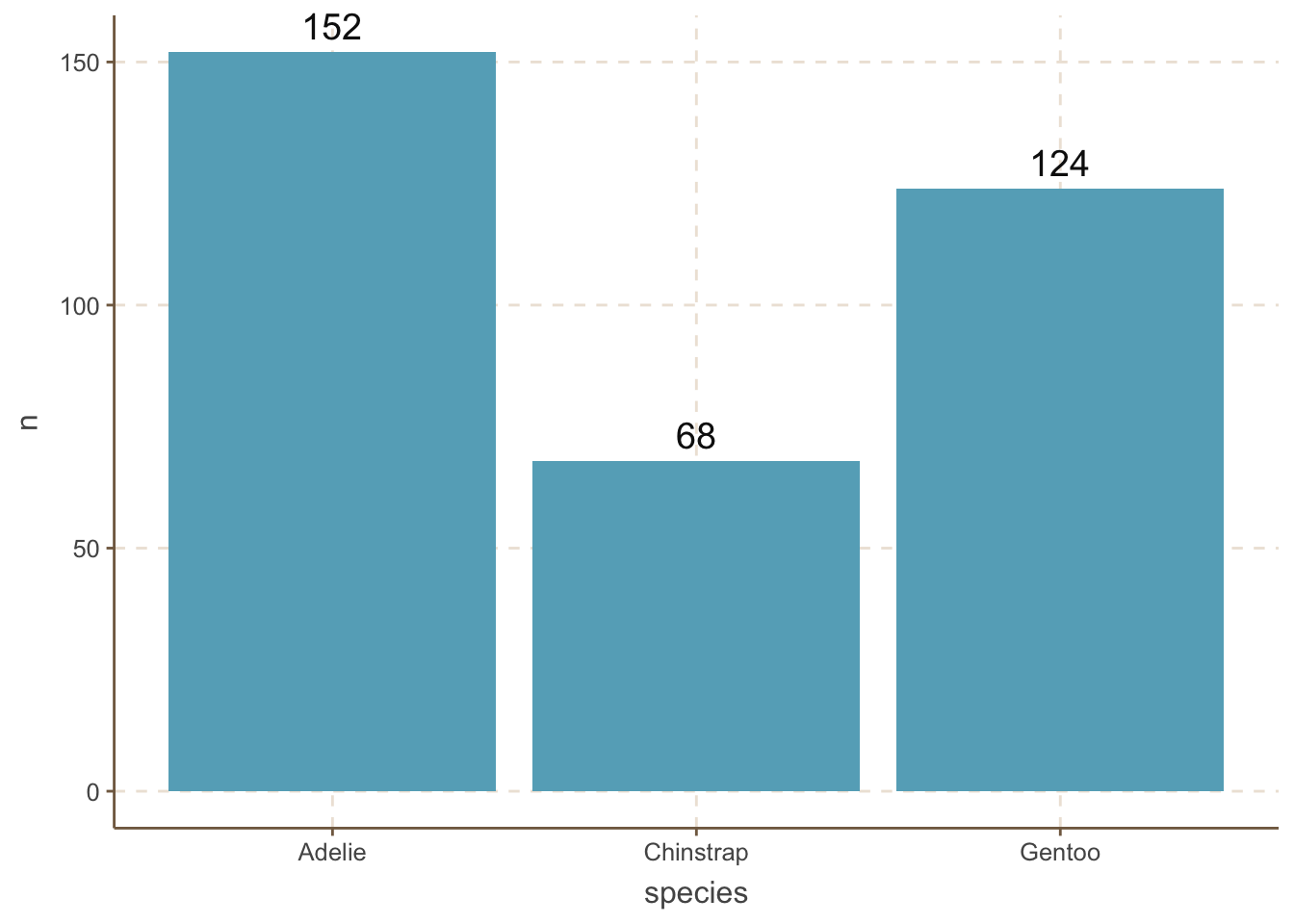
Two important things to note here:

The vjust argument in geom_text() is used to adjust the vertical position of the text label.
The coord_cartesian(clip = 'off') function is used to ensure that the text label is not clipped when it extends beyond the plot area. This is an important trick to remember.

It is helpful to reorder the bars in a bar plot. We can do this by using the reorder() function.

penguins_count |> 
    ggplot(aes(
        x = reorder(species, n),
        y = n
    )) + 
    geom_col() +
    geom_text(aes(label = n), size = 5, vjust = -0.5) +
    coord_cartesian(clip = 'off')

1: This tells ggplot to reorder the bars by the n column.

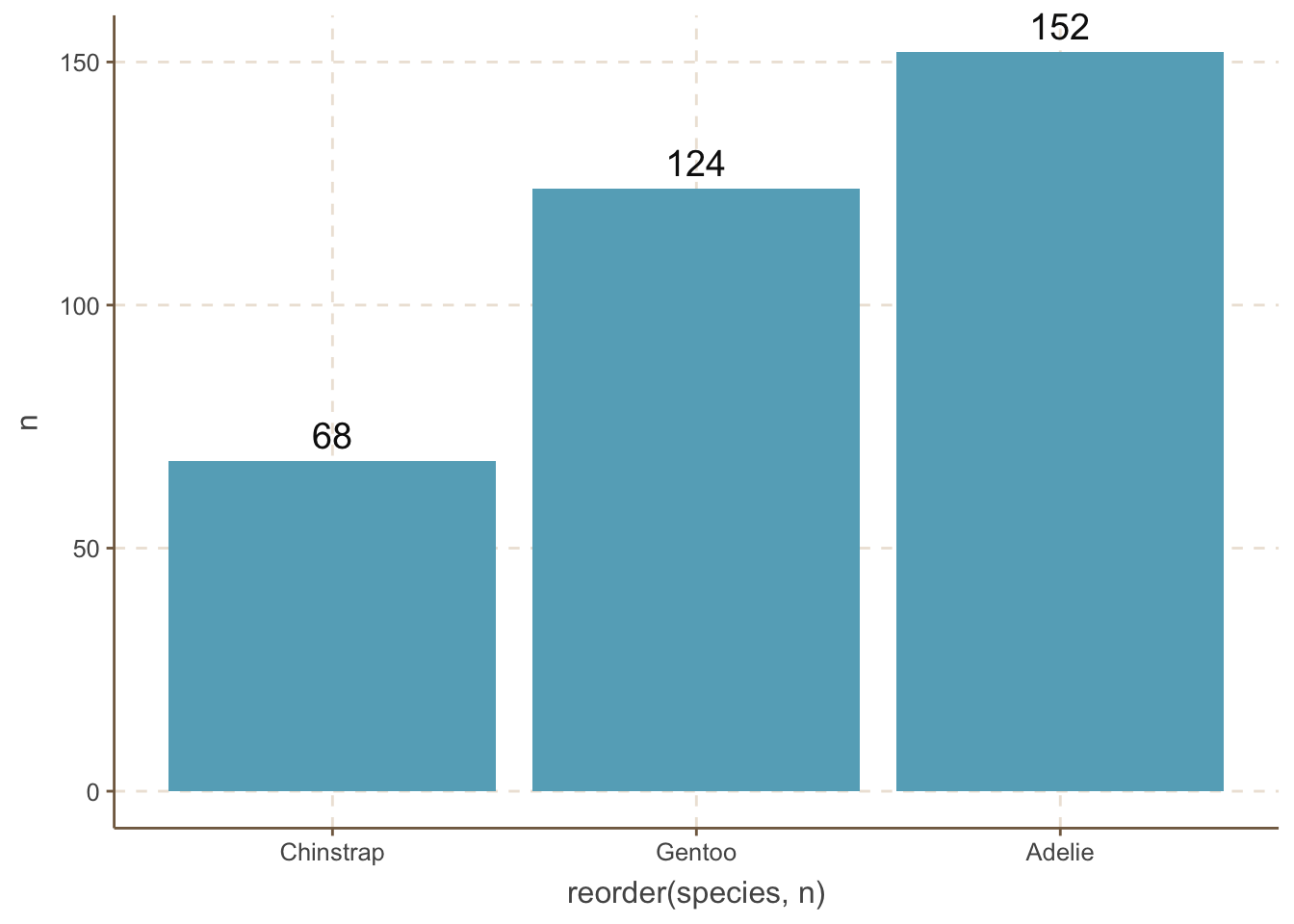
However, we do not always want to reorder the bars by the amount. For example, the categories are age distribution. When you want to reorder the bars by some manual order, you can use the fct_relevel() function.

penguins_count |> 
    mutate(species = fct_relevel(species, "Adelie", "Chinstrap", "Gentoo")) |>
    ggplot(aes(x = species, y = n)) +
    geom_col() +
    geom_text(aes(label = n), size = 5, vjust = -0.5) +
    coord_cartesian(clip = 'off')

1: This tells R to reorder the species column by the order of “Adelie”, “Chinstrap”, “Gentoo”.

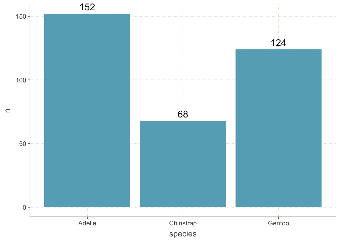
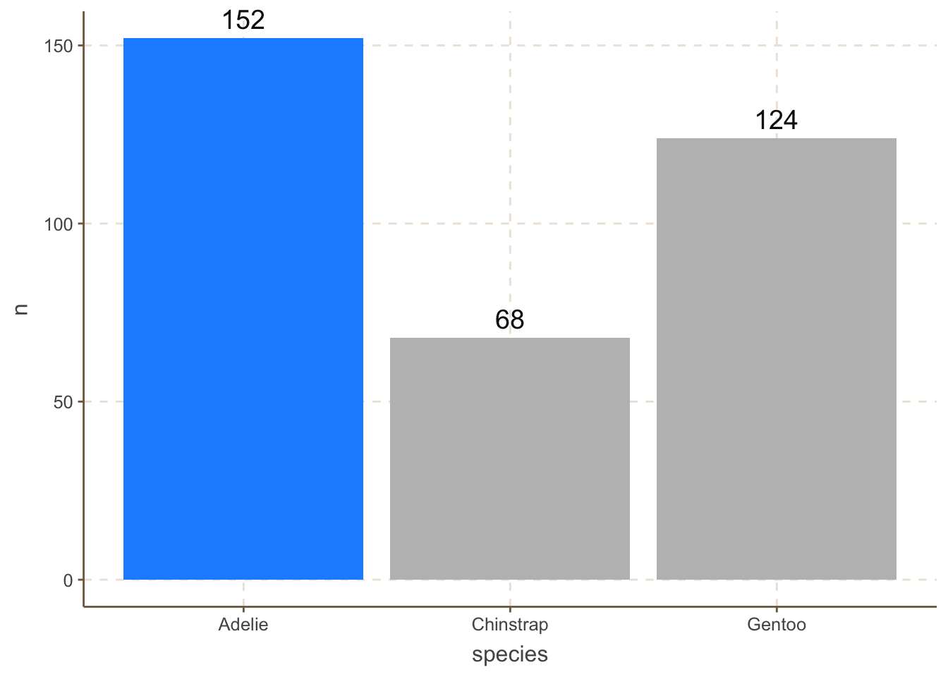
For example, we can highlight the “Adelie” category by changing its color to blue and graying out the others:

penguins_count |> 
    mutate(hl = species == "Adelie") |>
    ggplot(aes(x = species, y = n, fill = hl)) +
    geom_col() +
    scale_fill_manual(values = c("grey", "dodgerblue"), guide = "none") +
    geom_text(aes(label = n), size = 5, vjust = -0.5) +
    coord_cartesian(clip = 'off')

1: Create a logical column that marks the category to highlight.
2: Map the two values (FALSE, TRUE) to grey and blue, and hide the legend.

We sometimes want to differentiate the bars as much as possible. One obvious way is to use different colors for each bar:

penguins_count |> 
    ggplot(aes(x = species, y = n, fill = species)) +
    geom_col() +
    geom_text(aes(label = n), size = 5, vjust = -0.5) +
    MetBrewer::scale_fill_met_d("Hiroshige", direction=1)+
    coord_cartesian(clip = 'off')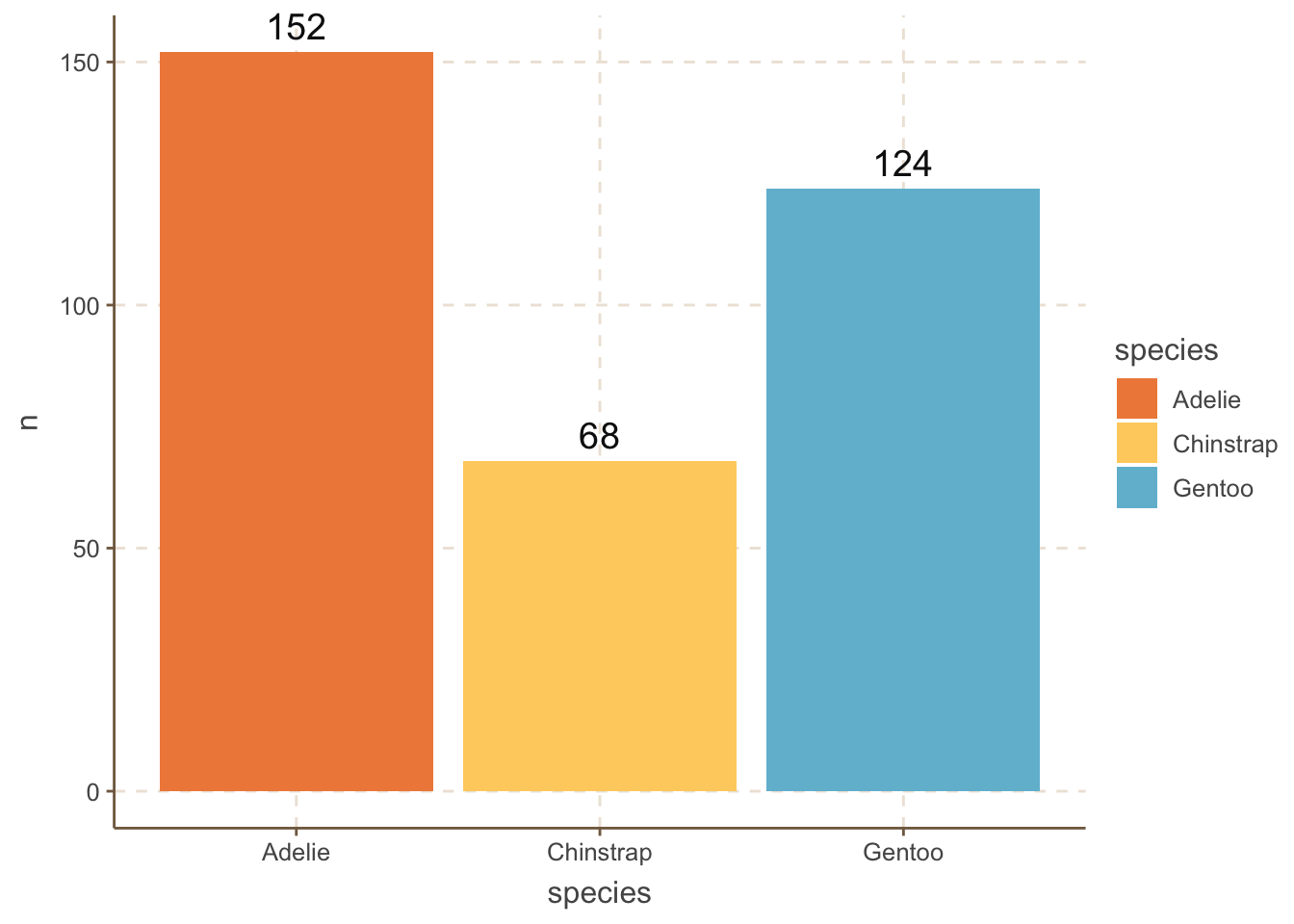

However, colors are not the only way, especially when people may print the plot in black and white. One alternative is to use different patterns for each bar using the ggpattern package.

penguins_count |> 
    ggplot(aes(x = species, y = n)) +
    ggpattern::geom_col_pattern(
        aes(pattern_fill = species, 
            pattern      = species), 
            fill  = 'white',
            color = 'black'
    ) +
    ggpattern::scale_pattern_discrete() +
    ggpattern::scale_pattern_fill_discrete() +
    geom_text(aes(label = n), size = 5, vjust = -0.5) +
    coord_cartesian(clip = 'off') +
    theme(legend.position = "none")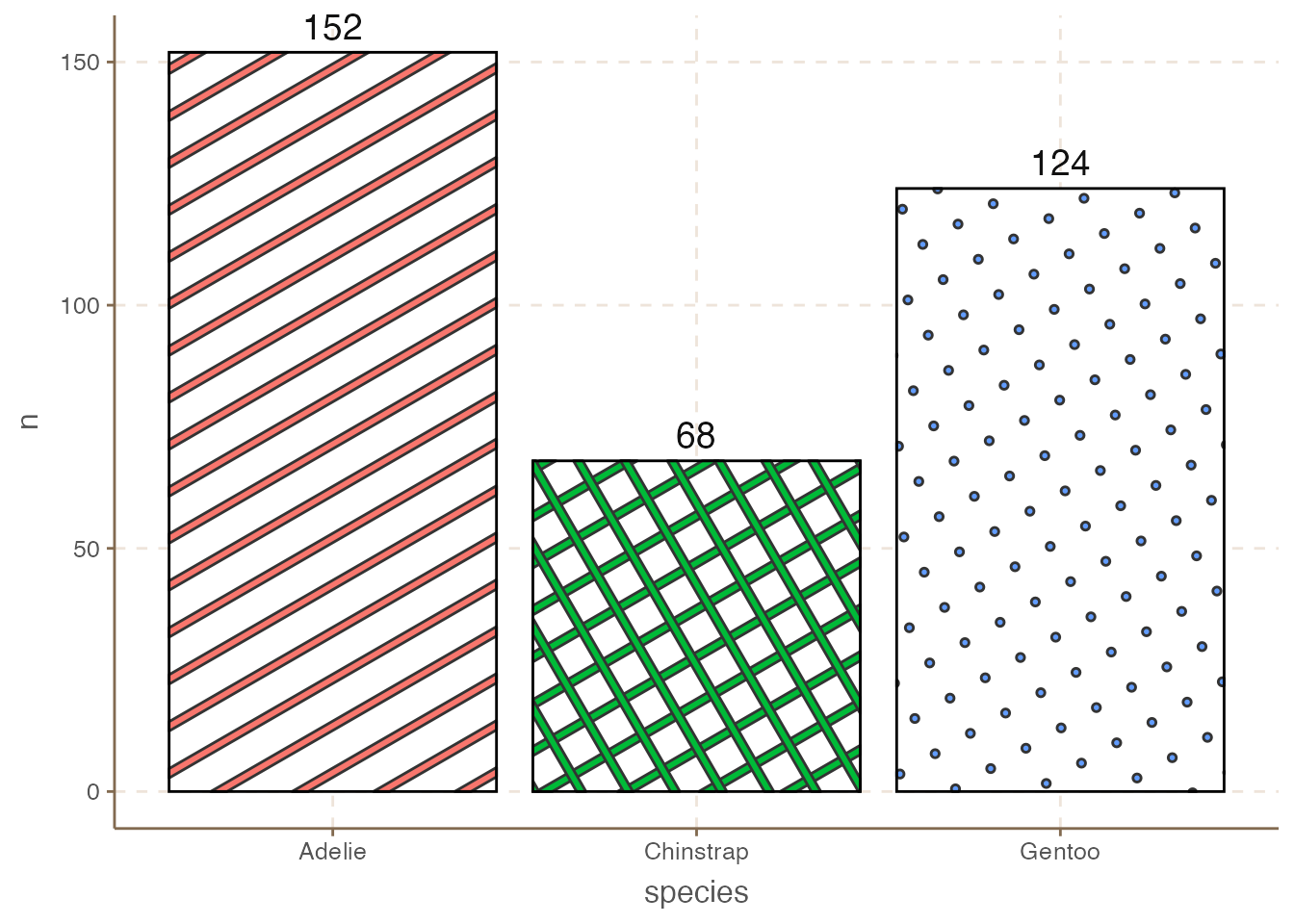

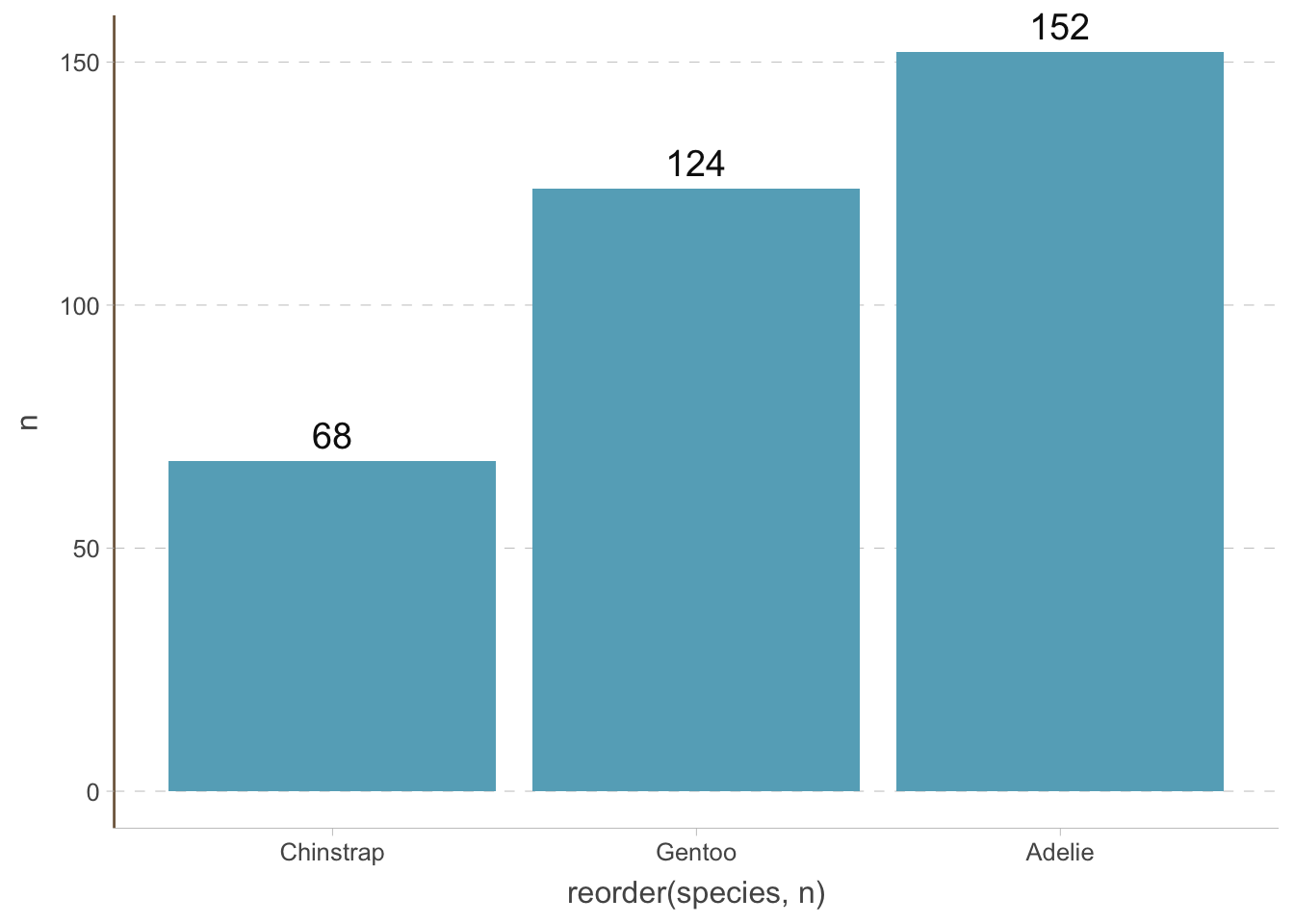
Since the bars are vertical, we do not need the vertical grid lines. We can change the theme of the plot by using the theme() function. Always think about what elements are redundant and remove them.

penguins_count |> 
    ggplot(aes(
        x = reorder(species, n),
        y = n
    )) + 
    geom_col() +
    geom_text(aes(label = n), size = 5, vjust = -0.5) +
    coord_cartesian(clip = 'off') +
    theme(
        axis.line.x = element_line(colour = "grey", linewidth = 0.15), 
        panel.grid.major.x = element_blank(), 
        panel.grid.minor.x = element_blank(), 
        panel.grid.major.y = element_line(colour = "grey", linewidth = 0.15), 
        panel.grid.minor.y = element_blank(), 
        axis.ticks.x = element_line(colour = "grey", linewidth = 0.15), 
        axis.ticks.y = element_line(colour = "grey", linewidth = 0.15)
    )

11.2 Bar plots variations

11.2.1 Horizontal bar plots

We can also create horizontal bar plots. This is useful when the category is a long string (rotating the x-axis text hurts readability; guides(x = guide_axis(n.dodge = 2)) or guide_axis(angle = 45) are milder alternatives). It is easy to do this by changing the x and y axis:

penguins_count |> 
    ggplot(aes(y = reorder(species, n), x = n)) +
    geom_col() +
    geom_text(aes(label = n), hjust = -0.3) +
    coord_cartesian(clip = 'off') +
    theme(
        axis.line.y = element_line(colour = "grey", linewidth = 0.15), 
        panel.grid.major.x = element_line(colour = "grey", linewidth = 0.15), 
        panel.grid.minor.x = element_blank(), 
        panel.grid.major.y = element_blank(), 
        panel.grid.minor.y = element_blank(), 
        axis.ticks.x = element_line(colour = "grey", linewidth = 0.15), 
        axis.ticks.y = element_line(colour = "grey", linewidth = 0.15)
    )

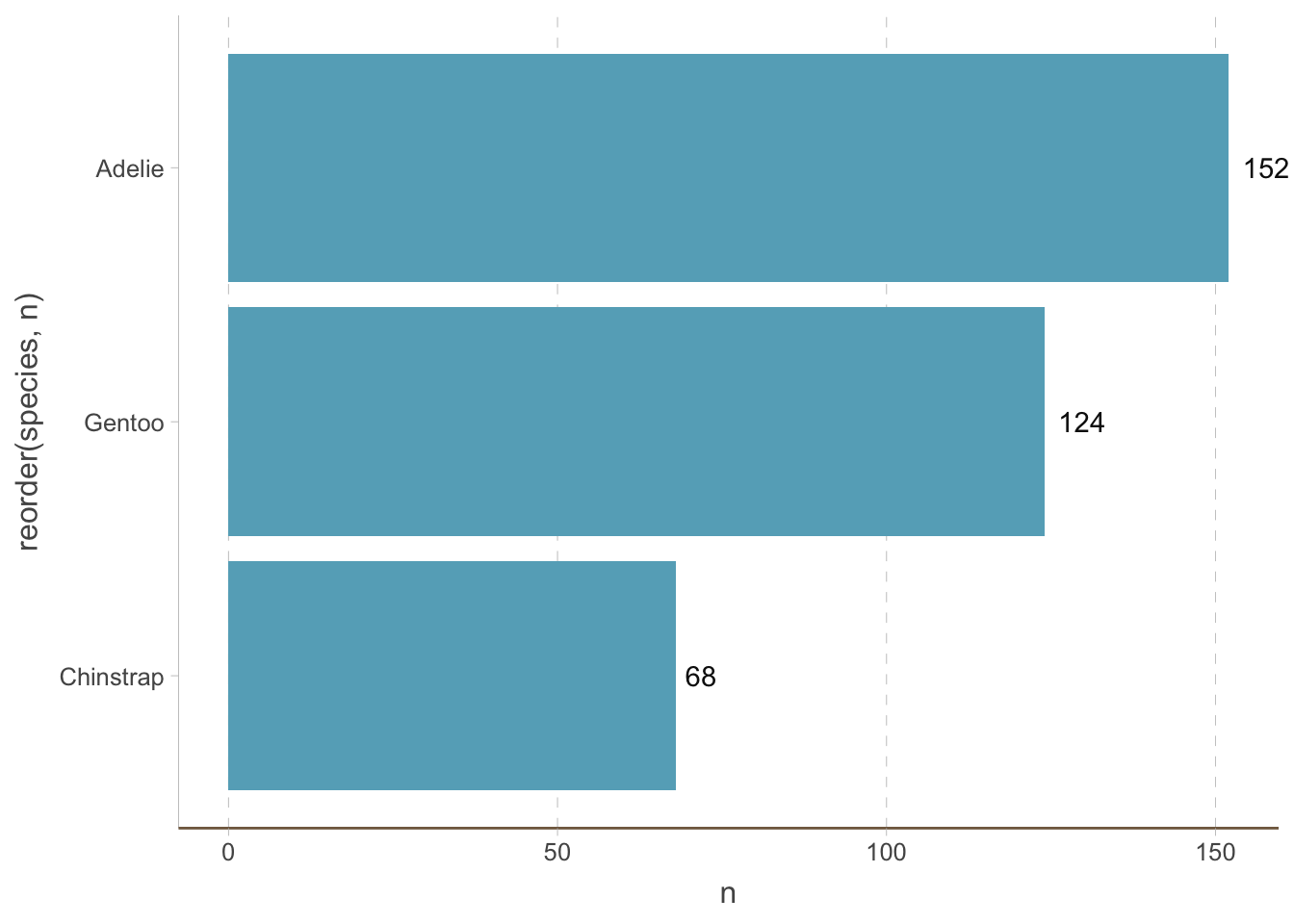
Notice that we have removed the horizontal (instead of vertical) grid lines because they are redundant now.

11.2.2 Lollipop plots

Bar plots are not the only way to visualize the amount of different categories. A big issue with bar plots is that it has a low data-to-ink ratio (This is not a principle we have to follow always, but it is helpful to keep in mind). Dot plots are a (increasingly popular) alternative.

We can create a dot plot by adding a shrunken bar plot and then adding points to it:

penguins_count |> 
    ggplot(aes(y = reorder(species, n), x = n)) +
    geom_col(width = 0.01) +
    geom_point(size = 5) +
    geom_text(aes(label = n), size = 5, vjust = -1) +
    coord_cartesian(clip = 'off') +
    theme(
        axis.line.y = element_line(colour = "grey", linewidth = 0.15), 
        panel.grid.major.x = element_line(colour = "grey", linewidth = 0.15), 
        panel.grid.minor.x = element_blank(), 
        panel.grid.major.y = element_blank(), 
        panel.grid.minor.y = element_blank(), 
        axis.ticks.x = element_line(colour = "grey", linewidth = 0.15), 
        axis.ticks.y = element_line(colour = "grey", linewidth = 0.15)
    )

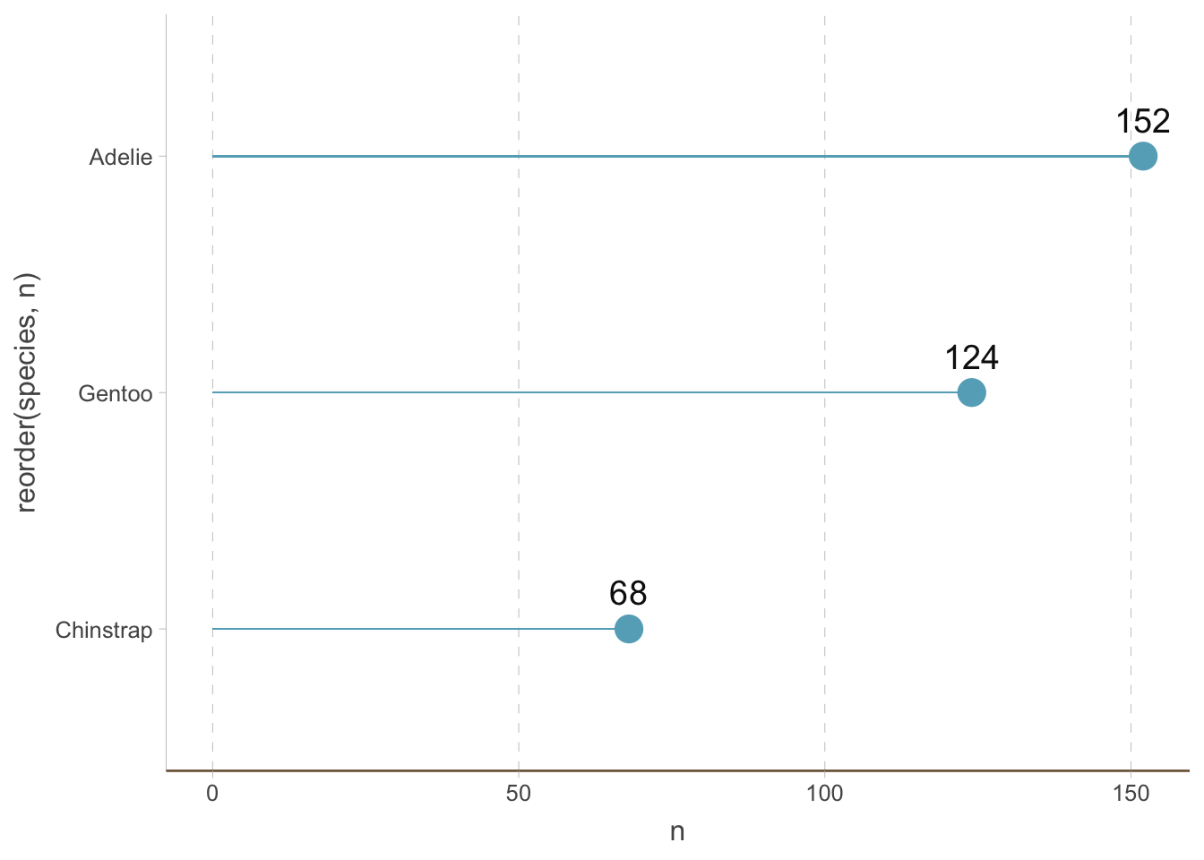
The ggalt package also provides geom_lollipop() as a shortcut for lollipop plots (see its documentation).

11.2.3 Circular bar plots

Another trendy way to visualize the amount of different categories is to use circular bar plots.

penguins_count |> 
    ggplot(
        aes(x = reorder(species, n), 
            y = n, 
            color = species, 
            fill = species
        )
    ) +
    geom_col(alpha = .5) +
    scale_y_continuous(
        limits = c(-50, 160)
    ) + 
    geom_hline(yintercept = 50, color = "grey", linewidth = 0.15) +
    geom_hline(yintercept = 100, color = "grey", linewidth = 0.15) +
    geom_hline(yintercept = 150, color = "grey", linewidth = 0.15) +
    geom_text(aes(label = species), position = position_stack(vjust = 0.5), color = 'white') +
    coord_polar() +
    theme_void() +
    theme(
        legend.position = "none"
    )

Warning: The `scale_name` argument of `discrete_scale()` is deprecated as of ggplot2
3.5.0.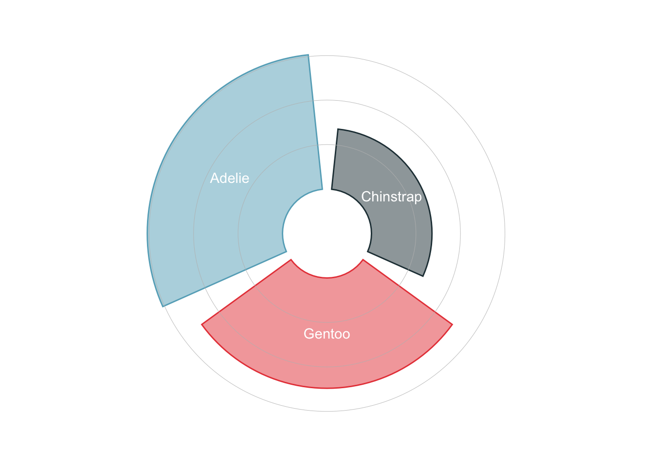

11.2.4 Waffle charts

It is also increasingly popular to use waffle charts to visualize the amount of different categories.

ggplot(penguins_count, aes(fill=species, values=n)) +
  waffle::geom_waffle(color = 'white') +
  theme_void()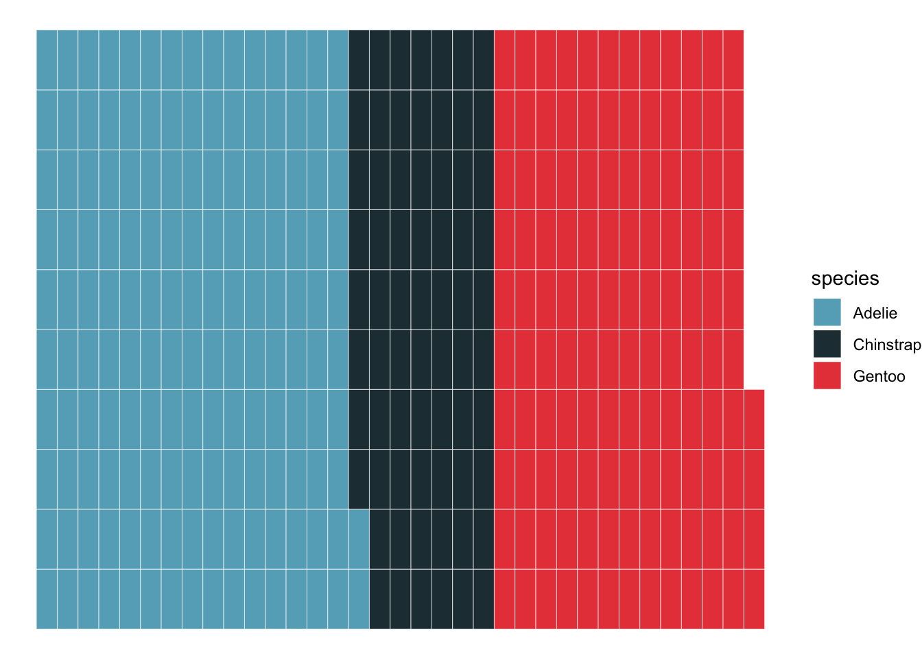

Parliament plots

penguins_count |>
    ggplot() +
    ggpol::geom_parliament(aes(seats = n, fill = species), color = "black") +
    scale_fill_manual(
        values = MetBrewer::met.brewer("Isfahan2", direction=1), 
        labels = c("Adelie", "Chinstrap", "Gentoo")) +
    theme_void()

Warning: Using the `size` aesthetic in this geom was deprecated in ggplot2 3.4.0.
ℹ Please use `linewidth` in the `default_aes` field and elsewhere instead.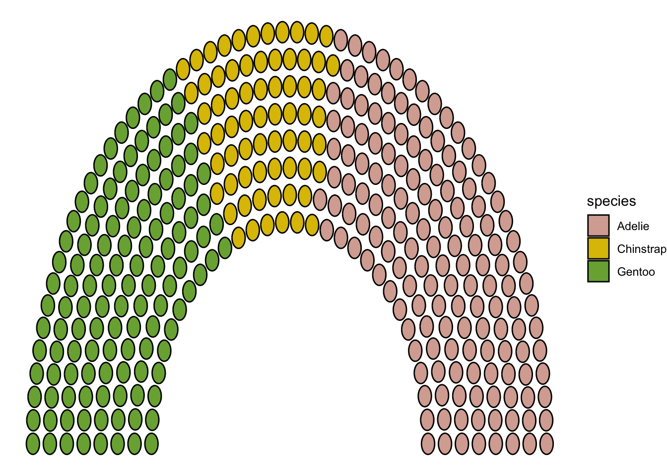

11.3 Treemaps: showing parts of a whole

A treemap divides a region into smaller tiles whose areas represent amounts. We will use the same penguins_count table as the bar plots above: each species contributes part of the 344 penguins recorded in this dataset. These are counts in the sample, not estimates of the species’ populations in the wild.

11.3.1 Rectangular treemaps

First, calculate each species’ share and make labels that include the count and percentage. Keeping the same data makes it easier to compare the treemap with the earlier bar plot.

penguins_treemap <- penguins_count |>
    mutate(
        share = n / sum(n),
        label = paste0(species, "\n", n, " penguins\n",
                       scales::percent(share, accuracy = 0.1))
    )

penguin_colors <- c(
    Adelie = "#66C2A5",
    Chinstrap = "#FC8D62",
    Gentoo = "#8DA0CB"
)

Use treemapify to map the counts to tile areas. We call its functions directly with package::function(), without attaching another package.

penguins_treemap |>
    ggplot(aes(area = n, fill = species, label = label)) +
    treemapify::geom_treemap(colour = "white") +
    treemapify::geom_treemap_text(
        place = "centre", colour = "black", size = 16
    ) +
    scale_fill_manual(values = penguin_colors, guide = "none") +
    theme_void() +
    labs(caption = "Each tile's area represents its share of the 344 sampled penguins.")

1: area = n makes tile area proportional to the count. The package calculates the layout; we do not set tile widths or heights ourselves.
2: Put the species, count, and percentage inside each tile. The text layer shrinks labels when needed to fit.

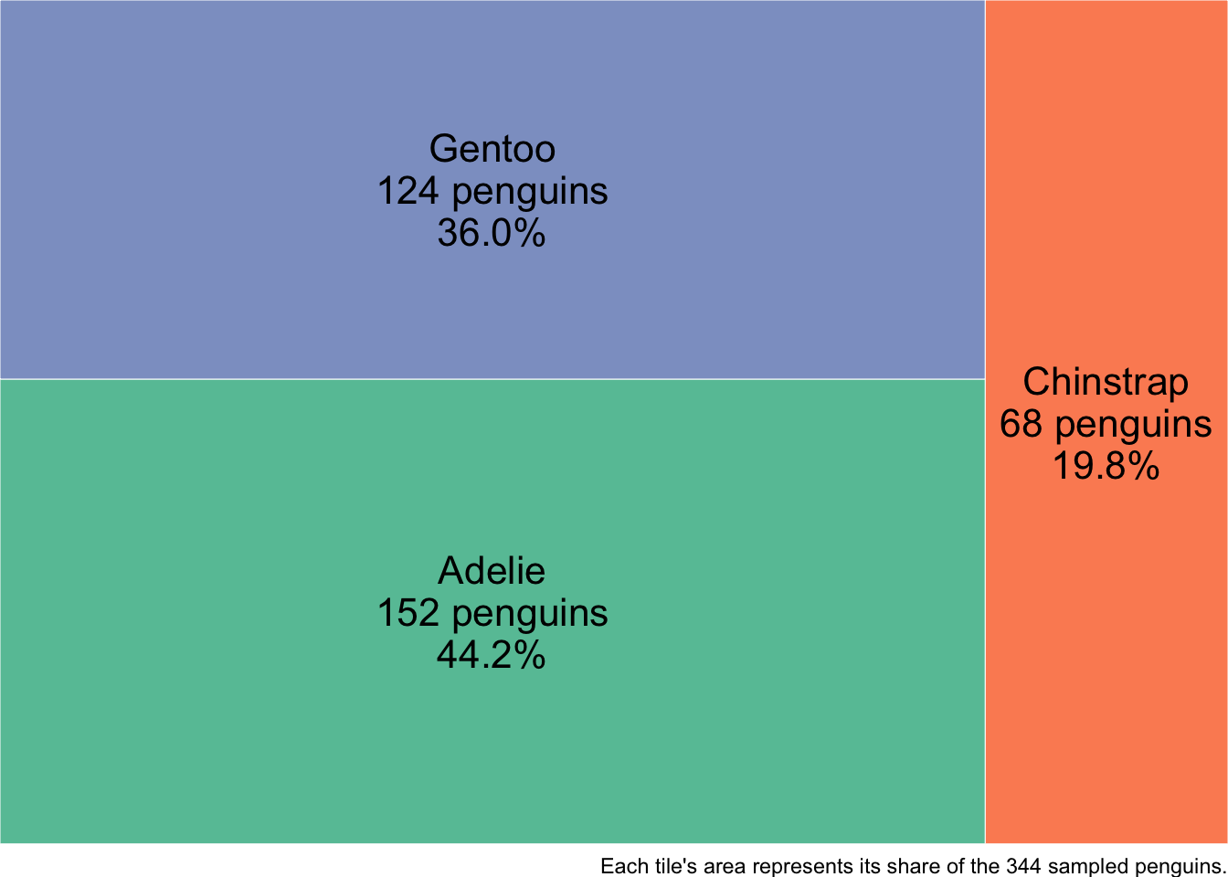
Adelie penguins make up about 44.2% of this sample, so their tile occupies about 44.2% of the plotting region. Color identifies the species; it does not encode another numerical variable.

11.3.2 Voronoi treemaps

A weighted Voronoi treemap uses irregular polygons instead of rectangles while retaining the same area encoding. We can make one with the penguin counts using WeightedTreemaps. Its layout function computes the polygons, and a separate function draws them.

penguins_voronoi <- WeightedTreemaps::voronoiTreemap(
    data = as.data.frame(penguins_treemap),
    levels = "label",
    cell_size = "n",
    shape = "rectangle",
    maxIteration = 500,
    error_tol = 0.001,
    seed = 234
)

WeightedTreemaps::drawTreemap(
    penguins_voronoi,
    color_palette = unname(penguin_colors),
    border_color = "white", border_size = 3,
    label_color = "black", label_size = 3, label_autoscale = FALSE
)

1: Each species has a distinct label, defining one cell in this single-level treemap.
2: Weight the cell areas by the counts. An ordinary, unweighted Voronoi diagram would not encode these amounts.
3: Fix the seed to make the layout reproducible. Polygon shapes and positions are layout choices; they do not represent additional measurements.

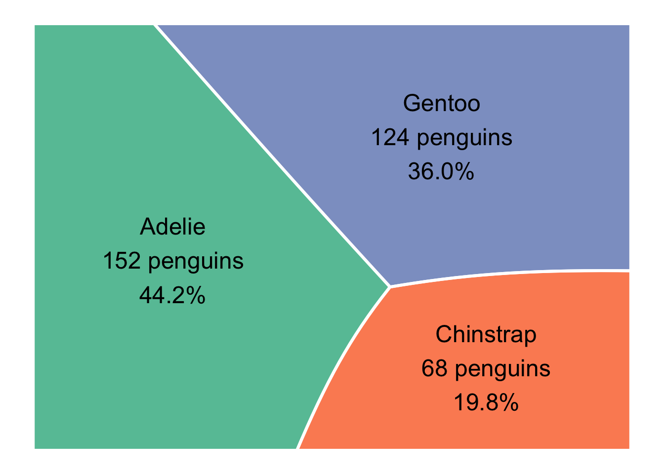
The two treemaps represent the same counts. The weighted layout approximates the target area proportions through an iterative calculation; the tolerance and iteration limit above control that calculation. Use the labels for exact values, and prefer bars when small differences between categories are the main question. With only three species, a bar plot is easy to read; treemaps become more useful when the question concerns composition or nested categories.

Optional extension: global biomass

To try a different application, use the authors’ biomass results spreadsheet and data and analysis repository for Bar-On, Phillips, and Milo (2018). The classroom examples above use only penguins.

Choose non-overlapping groups and a common biomass unit, then replace penguin counts with those amounts. If you expand a small category into a second panel, as in Figure 1B of the paper, label that panel’s total explicitly: its areas are normalized to a different whole and cannot be compared directly with areas in the overview.

11.4 Multiple categories

How about multiple types of categories? Suppose we want to visualize the amount of penguins of different species and sex. Let us first count the number of penguins of each species and sex:

penguins_count_sex <- penguins |>
    drop_na(sex) |>
    group_by(species, sex) |>
    summarise(n = n(), .groups = "drop")

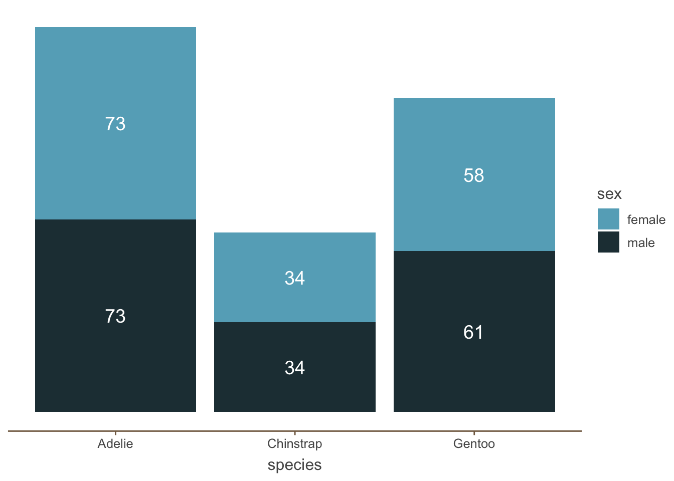
The most obvious way to visualize this is to use bar plots.

Stacked bar plots
Side by side bar plots

Stacked bar plots are a very common way to visualize the amount of different categories. However, it is hard to compare the amounts of the lower segments across species, because they do not share a common baseline.

penguins_count_sex |>
    ggplot(aes(x = species, y = n, fill = sex)) +
    geom_col()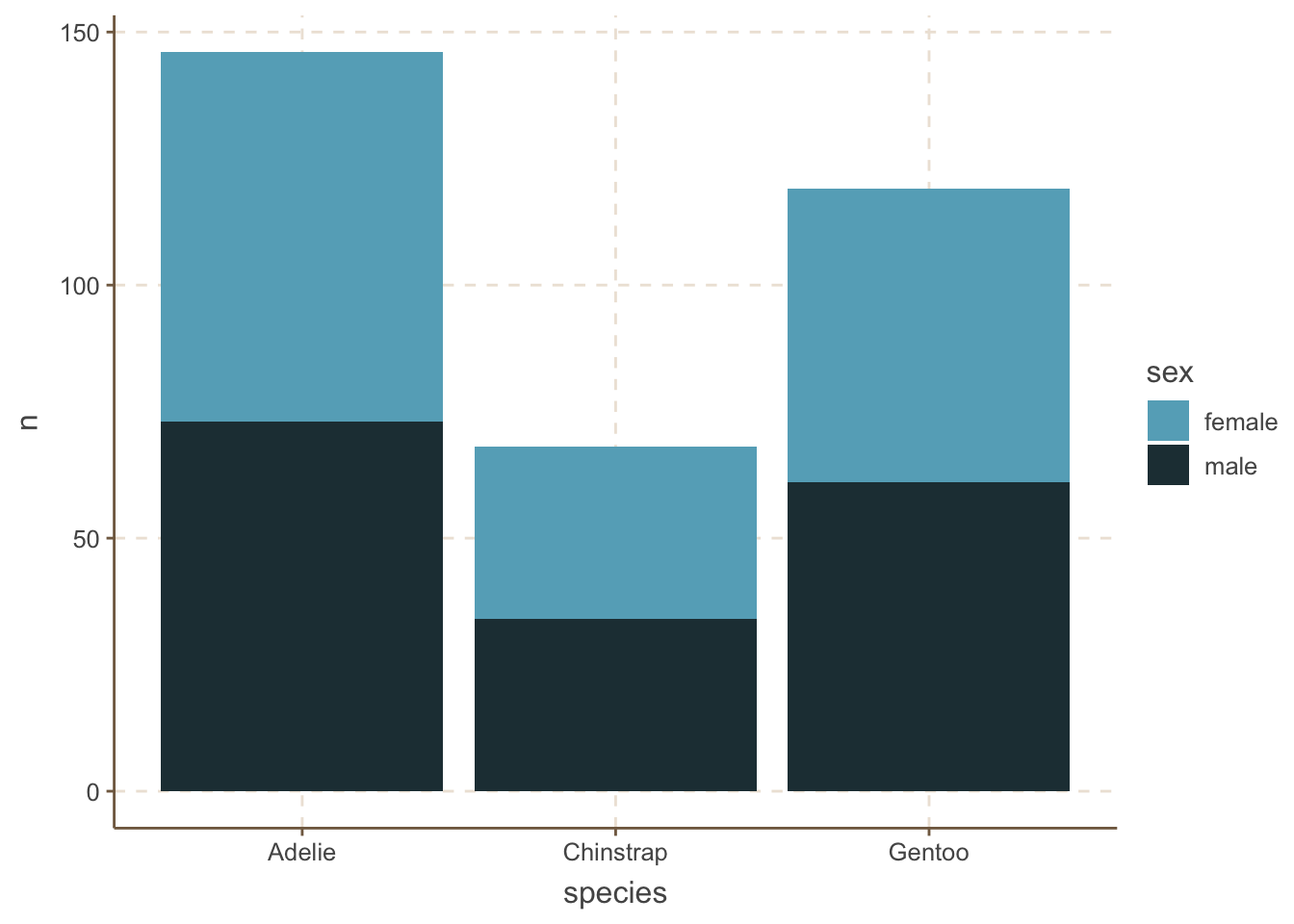

One potential solution is to remove the y axis and just add the amount of each category:

penguins_count_sex |>
    ggplot(aes(x = species, y = n, fill = sex)) +
    geom_col() +
    geom_text(
        aes(label = n), 
        color = 'white',
        size = 5,
        position = position_stack(vjust = 0.5)) +
    theme(
        axis.line.y = element_blank(), 
        panel.grid.major = element_blank(), 
        panel.grid.minor = element_blank(), 
        axis.ticks.y = element_blank(),
        axis.text.y = element_blank(),
        axis.title.y = element_blank()
    )

An alternative to stacked bar plots is to plot the bars side by side. This is useful when you want to compare the amounts of the sexes within each species.

penguins_count_sex |>
    ggplot(aes(x = species, y = n, fill = sex)) +
    geom_col(position = "dodge")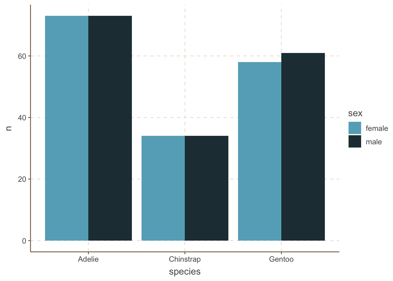

11.4.1 Waffle charts

You can also use other types (geoms) as well. For example, waffle charts.

penguins_count_sex |>
    ggplot(aes(values = n, fill = sex)) +
    waffle::geom_waffle(color = "white", linewidth = .25, n_rows = 10, flip = TRUE) +
    facet_wrap(~species, nrow = 1, strip.position = "bottom") +
    scale_x_discrete() +
    MetBrewer::scale_fill_met_d("Hiroshige", direction=1)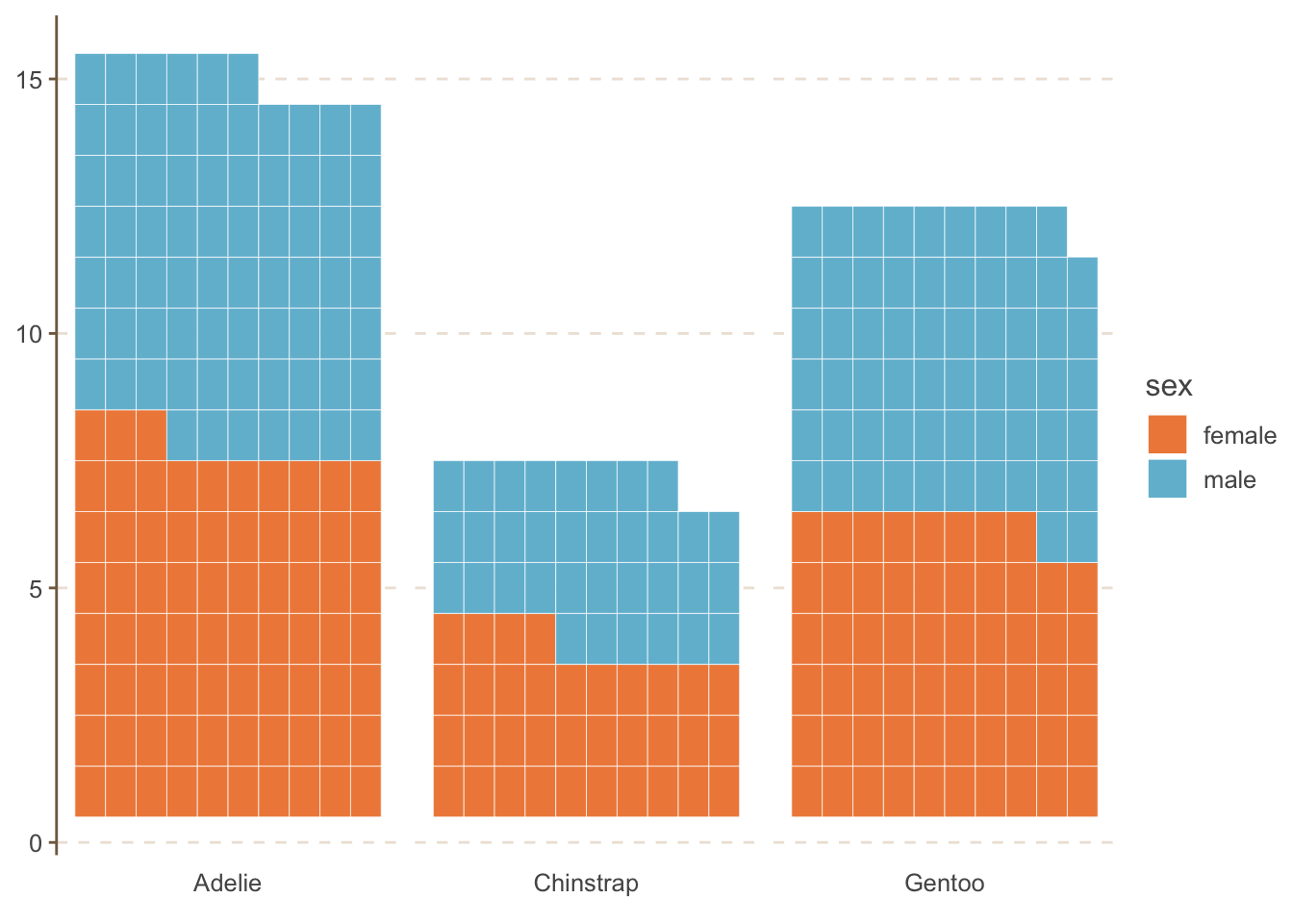

11.4.2 Dumbbell plots

Another useful alternative is to use the dumbbell plot. It is quite similar to the lollipop plot. We will use the ggalt package to create the dumbbell plot.

penguins |>
    drop_na(sex) |>
    group_by(species, sex) |>
    summarise(mean_bill_length = mean(bill_length_mm, na.rm = TRUE), .groups = "drop") |>
    pivot_wider(names_from = sex, values_from = mean_bill_length) |>
    ggplot(aes(x = female, xend = male, y = species)) +
    ggalt::geom_dumbbell(size=3, color="#e3e2e1", 
                colour_x = "#5b8124", colour_xend = "#bad744",
                dot_guide=TRUE, dot_guide_size=0.5) +
    labs(x=NULL, y=NULL) +
    hrbrthemes::theme_ipsum_rc(grid="X")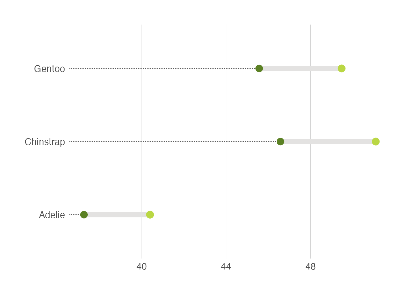

ggalt::geom_dumbbell() still uses the old size argument for the segment width (it ignores linewidth), so recent versions of ggplot2 print a deprecation warning here. The plot is unaffected.