17 Additional Topics in Data Visualization

Class Objectives

Combine multiple plots using the awesome patchwork package.
Make interactive plots to let your audience dive into your data.
Create animated visualizations and step-by-step reveals to show patterns and changes over time.

Packages for this chapter

If you haven’t installed the following packages, run this code:

pak::pak(c("patchwork", "plotly", "ggiraph", "gganimate", "ggreveal", "dygraphs"))

You’ve done great exploring data visualization so far. Now, let’s dive into some exciting extras that’ll really make your visualizations stand out—perfect for your papers, presentations, or blog posts!

17.1 Combining Plots with `patchwork`

Did you know that many academic journals limit the number of figures per paper? To squeeze more information into fewer figures, you can combine multiple plots into one tidy visual (just a random example I found online). The easiest and most intuitive way to do this is with the patchwork package—seriously, once you try it, you’ll never go back!

library(tidyverse)
library(patchwork)
library(palmerpenguins)

# First plot: Scatter plot
p1 <- ggplot(penguins, aes(x = bill_length_mm, y = bill_depth_mm, color = species)) +
    geom_point(alpha = 0.7) +
    theme_minimal()

# Second plot: Density plot
p2 <- ggplot(penguins, aes(x = flipper_length_mm, fill = species)) +
    geom_density(alpha = 0.5) +
    theme_minimal()

Use the + operator to combine plots horizontally:

p1 + p2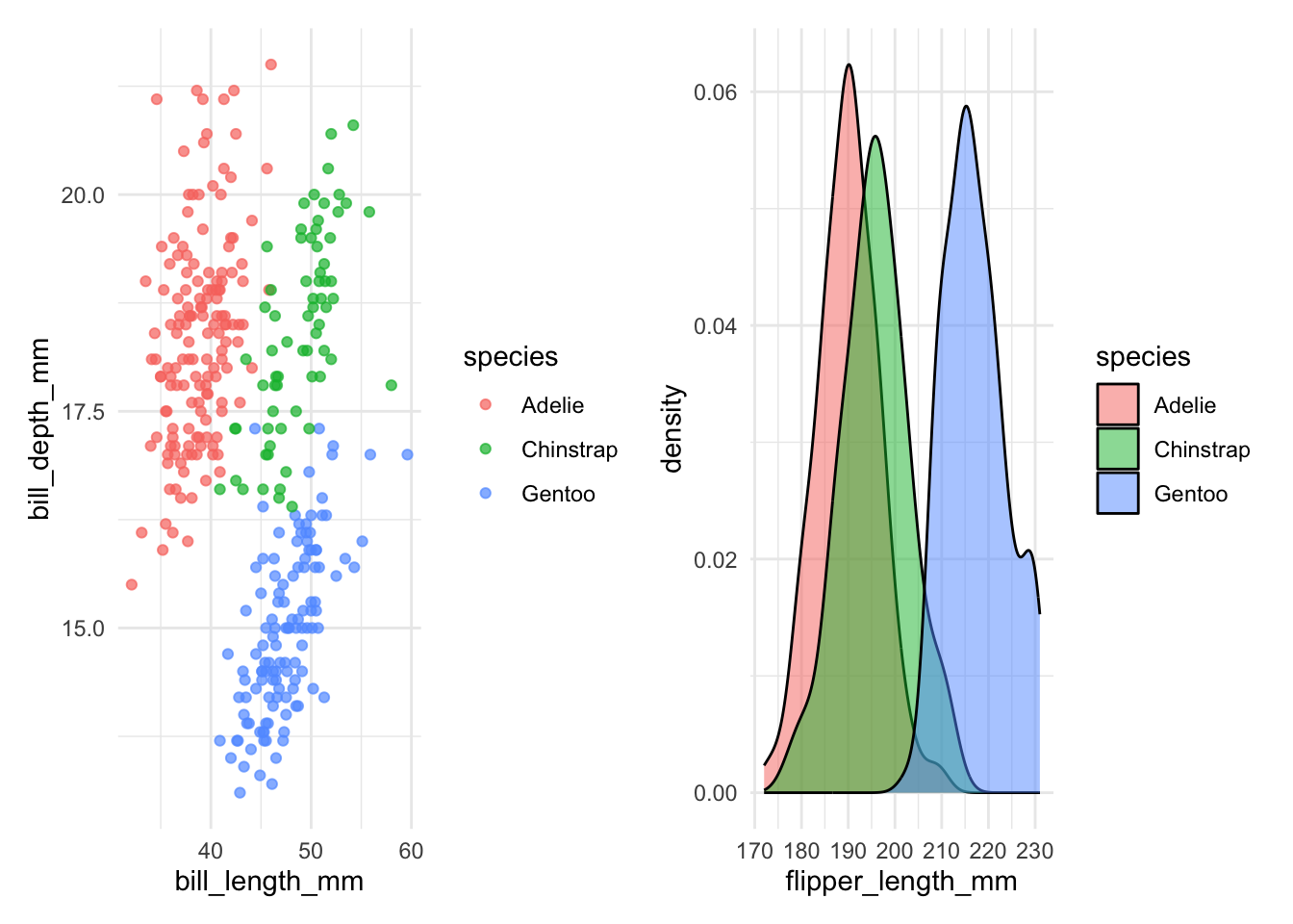

Use the / operator to combine plots vertically:

p1 / p2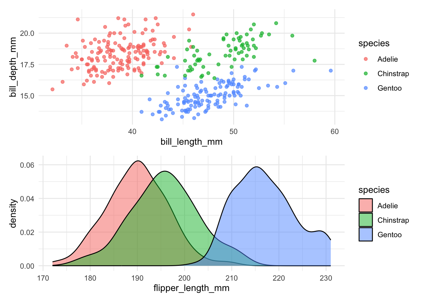

Combine multiple plots in a single line of code:

p3 <- ggplot(penguins, aes(x = species, y = body_mass_g)) +
    geom_boxplot(aes(fill = species)) +
    labs(title = "Body Mass by Species") +
    theme_minimal()

(p1 | (p2 / p3))

1: Complex layout: p1 on the left; p2 above p3 on the right

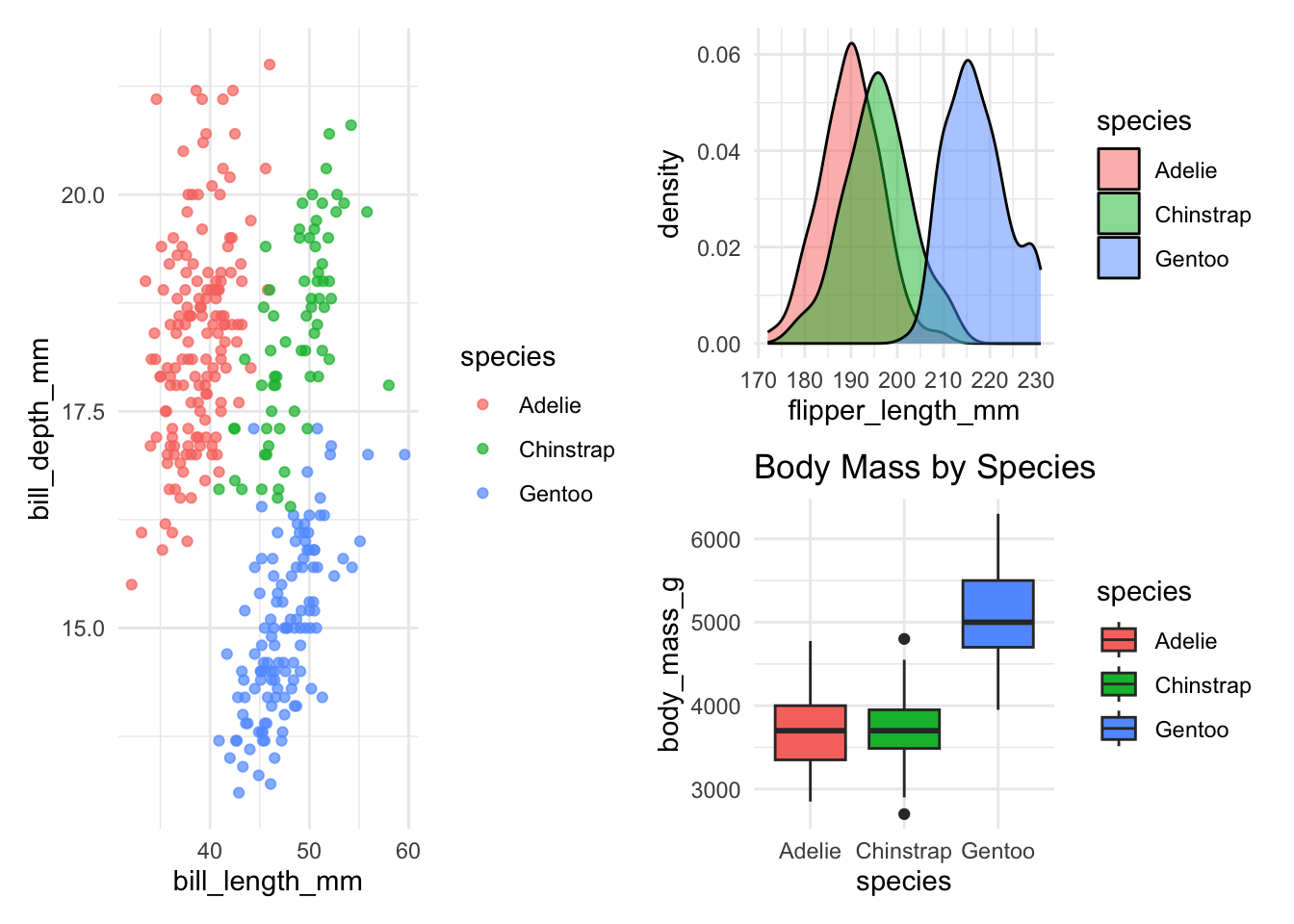
Let’s explore the advanced features of patchwork with one practical example:

p1 +
  (p2 + guides(fill = "none")) +
  plot_layout(
    widths = c(5, 2)
  ) +
  plot_layout(guides = "collect") +
  plot_annotation(
    tag_levels = "A"
  ) &
  theme_minimal()

1: Remove the fill legend from the second plot (p2)
2: Set the widths of the two plots in a 5:2 ratio (the left plot takes about 71% of the width)
3: Tag the panels with letters: A, B, and so on
4: The & operator applies the theme to every subplot in the composition (a plain + would only affect the last plot)

17.2 Creating Interactive Plots

Unfortunately, interactive plots can’t be included in traditional academic papers (bummer!), but they’re incredibly effective for presentations, blogs, or web-based content, letting viewers actively explore your data.

17.2.1 plotly

Plotly offers the easiest way to turn a ggplot2 static figure to an interactive version. Just plot as always, then use ggplotly() to convert it to an interactive plot.

library(plotly)

# Create basic ggplot as usual
p_plotly <- penguins |> 
    ggplot(aes(x = bill_length_mm, y = bill_depth_mm, color = species)) +
    geom_point(
        aes(text = paste(
            "Species:", species, 
            "<br>Island:", island,
            "<br>Body mass:", body_mass_g, "g"
        )),
        alpha = 0.7
    ) +
    theme_minimal() 

# Convert to plotly
ggplotly(p_plotly, tooltip = "text")

1: is used to create a line break in the tooltip

Figure 17.1: Interactive plot with hover data using plotly

17.2.2 ggiraph

While plotly gives you interactivity for free, ggiraph gives you interactivity with control. It is the tool of choice when you need precise customization — custom hover styles, linked highlighting across plots, and the ability to combine interactive plots with patchwork.

The key idea is simple: you swap standard ggplot2 geoms for their interactive counterparts (e.g., geom_point() → geom_point_interactive()), and then render the result with girafe() instead of printing it directly.

The Two Key Aesthetics

Every interactive geom in ggiraph understands two special aesthetics:

Aesthetic	What it does
`tooltip`	The text that pops up when you hover over an element. Supports HTML (e.g., `<b>`, `<br>`).
`data_id`	A linking key. All elements that share the same `data_id` light up together on hover.

Think of tooltip as the “what does this point say?” and data_id as the “what group does this point belong to?”

17.2.2.1 Basic Example: Tooltips + Linked Highlighting

Let’s build an interactive scatter plot. When you hover over any Adélie penguin, all Adélie penguins light up — and every other species fades out:

library(ggiraph)

p_ggiraph <- penguins |> 
    drop_na() |>
    ggplot(aes(x = bill_length_mm, y = bill_depth_mm, color = species)) +
    geom_point_interactive(
        aes(
            tooltip = paste( 
                "<b>Species:</b>", species, 
                "<br><b>Bill length:</b>", bill_length_mm, "mm", 
                "<br><b>Bill depth:</b>", bill_depth_mm, "mm" 
            ), 
            data_id = species
        ),
        size = 3, alpha = 0.7
    ) +
    theme_minimal()

girafe(
    ggobj = p_ggiraph,
    options = list(
        opts_hover(css = "fill:black;stroke:black;r:5pt;"),
        opts_hover_inv(css = "opacity:0.1;"),
        opts_zoom(max = 5)
    )
)

1: data_id = species links all points of the same species — hover one, highlight them all.
2: opts_hover() styles the highlighted elements (here: turn black and grow to a 5pt radius; note that changing r through CSS is not supported consistently across browsers).
3: opts_hover_inv() styles everything else (here: fade to 10% opacity).
4: opts_zoom() enables mouse-wheel zooming, up to 5×.

Figure 17.2: Hover over any point — all penguins of the same species will highlight together

Customizing the Hover Experience

The opts_hover() and opts_hover_inv() functions accept any valid CSS. Some useful patterns:

Enlarge on hover: "r:8pt;" (for points) or "stroke-width:3px;" (for lines)
Change color: "fill:gold;stroke:orange;"
Dim the rest: "opacity:0.05;" (very faint) or "filter:grayscale(100%);" (greyed out)

17.2.2.2 Linked Highlighting Across Multiple Plots

Here’s where ggiraph truly shines. When you combine multiple plots with patchwork and give them the same data_id, hovering in one plot instantly highlights the matching data in all the others. This is called linked highlighting (true brushing, where you drag a selection rectangle, is also possible with opts_selection()), and it’s incredibly powerful for exploring multivariate data.

Try it below — hover over a species cluster in the left panel and watch the right panel respond:

library(patchwork)

# Left panel: Bill morphology
p_bill <- penguins |>
    drop_na() |>
    ggplot(aes(x = bill_length_mm, y = bill_depth_mm, color = species)) +
    geom_point_interactive(
        aes(
            tooltip = paste("Species:", species),
            data_id = species
        ),
        size = 2.5, alpha = 0.6
    ) +
    labs(x = "Bill length (mm)", y = "Bill depth (mm)") +
    theme_minimal() +
    theme(legend.position = "none")

# Right panel: Body size
p_size <- penguins |>
    drop_na() |>
    ggplot(aes(x = flipper_length_mm, y = body_mass_g, color = species)) +
    geom_point_interactive(
        aes(
            tooltip = paste("Mass:", body_mass_g, "g"),
            data_id = species
        ),
        size = 2.5, alpha = 0.6
    ) +
    labs(x = "Flipper length (mm)", y = "Body mass (g)") +
    theme_minimal()

girafe(
    ggobj = p_bill + p_size,
    width_svg = 10, height_svg = 4,
    options = list(
        opts_hover(css = "opacity:1;"), 
        opts_hover_inv(css = "opacity:0.1;")
    )
)

1: The same data_id = species appears in both plots — this is what links them.
2: patchwork’s + operator combines the plots; girafe() renders them as a single interactive SVG.

Figure 17.3: Linked highlighting — hover in one plot, highlight in both

dygraphs for time series

A great tool for interactive time series plots is the dygraphs package. It allows you to zoom in and out of the time series, highlight specific time periods, and display additional information on hover. It has a different syntax than ggplot2, but it’s worth learning if you work with time series data.

17.3 Animated Visualizations and Reveals

Animations are awesome for illustrating changes over time or differences between groups. They’re engaging and clearly communicate your story, especially during presentations.

gganimate
ggreveal

Smoothly animate plots over continuous changes (like time). The key new function is transition_reveal() which reveals data points, lines (or other geom) over time. (The chunk below is not evaluated when this book is built; run it yourself to see the animation.)

library(gganimate)

economics  |> 
    ggplot(aes(x = date, y = unemploy / 1000)) +
    geom_line(linewidth = 1, color = "#0072B2") +
    geom_point(color = "white", fill = "#0072B2", shape = 21, size = 4) +
    transition_reveal(date) +
    labs(title = "Number of Unemployed People Over Time", y = "Unemployed (millions)") +
    theme_minimal()

1: Transition the plot by revealing data points over time

To save the animation as a GIF, use the anim_save() function.

ggreveal is not an animation tool. It creates a series of static plots that show how a figure is built step by step, which is handy for slides. For discrete groups, this is sometimes easier than animating.

library(ggreveal)

p <- penguins |> 
    filter(!is.na(sex))  |> 
    ggplot(aes(body_mass_g, bill_length_mm,
               group=sex, color=sex)) +
    geom_point() +
    geom_smooth(method="lm", formula = 'y ~ x', linewidth=1) +
    facet_wrap(~species) +
    theme_minimal()

reveal_groups(p)

17.1 Combining Plots with patchwork

17.2 Creating Interactive Plots

17.2.1 plotly

17.2.2 ggiraph

17.2.2.1 Basic Example: Tooltips + Linked Highlighting

17.2.2.2 Linked Highlighting Across Multiple Plots

17.3 Animated Visualizations and Reveals

17.1 Combining Plots with `patchwork`