pak::pak(c("colorspace", "ggnewscale", "palmerpenguins", "jtools"))16 Choosing Colors
Packages for this chapter
If you haven’t installed the following packages, run this code:
Effective use of color in data visualization is crucial for communicating your message clearly. However, color is inherently subjective—it varies by person, culture, and even across generations. While no single “perfect” color scheme exists, following some general guidelines can help you create more readable, appealing, and accessible graphics.
16.1 What to consider?
As mentioned in Chapter 6, you can have a lot of fun with choosing color palettes (e.g., MetBrewer). However, there are caveats you need to be aware of.
16.1.1 Think about the nature of the variable
First thing, before selecting a color palette, determine the nature of the variable you want to display. Two things matter: the data type (discrete, continuous, or binned) and the palette type (qualitative, sequential, or diverging). The tabs below walk through the most common combinations. Note that sequential and diverging palettes also apply to discrete or binned data: an ordered variable such as low/medium/high should get a sequential palette (e.g., scale_fill_discrete_sequential()), not a qualitative one.
Use distinct colors for each category. For example, we want to use color to distinguish the species of penguins.
Show the code
library(tidyverse)
library(palmerpenguins)
library(colorspace)
ggplot(penguins, aes(x = bill_length_mm, y = bill_depth_mm, fill = species)) +
    geom_point(shape = 21, color = "white", alpha = 0.5, size = 3) +
    scale_fill_discrete_qualitative() +
    labs(x = "Bill Length (mm)", y = "Bill Depth (mm)") +
    jtools::theme_nice() +
    theme(legend.position = "top")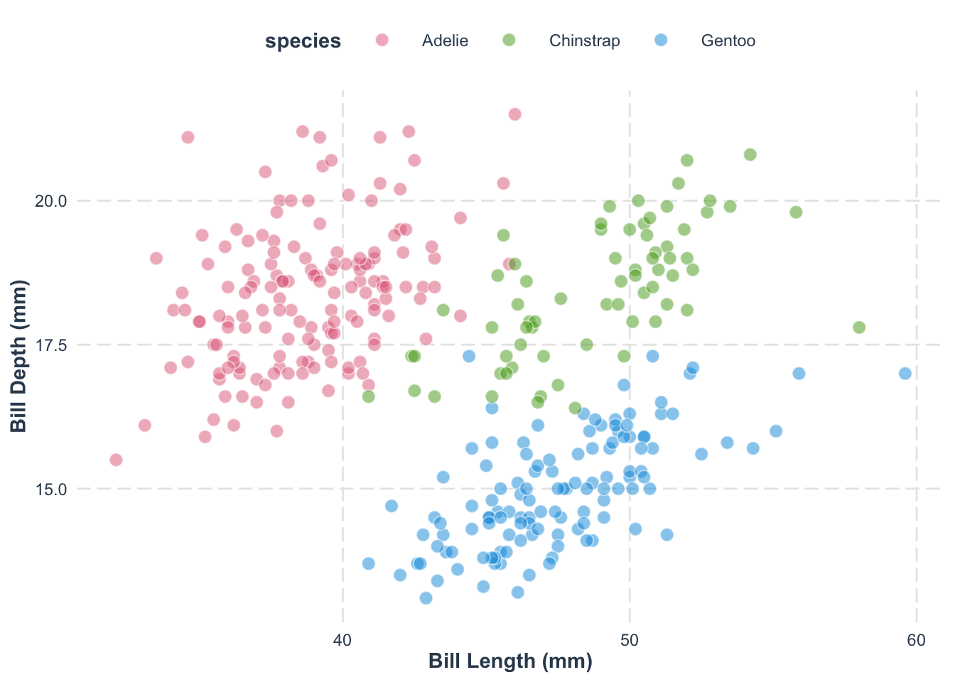
For variables with an inherent order, choose a palette that represents a gradual change. For example, we want to use the color to indicate the body mass of penguins.
Show the code
library(tidyverse)
library(palmerpenguins)
library(colorspace)
ggplot(penguins, aes(x = bill_length_mm, y = bill_depth_mm, fill = body_mass_g)) +
    geom_point(shape = 21, color = "white", alpha = 0.7, size = 3) +
    scale_fill_continuous_sequential() +
    labs(x = "Bill Length (mm)", y = "Bill Depth (mm)") +
    jtools::theme_nice() +
    theme(legend.position = "top")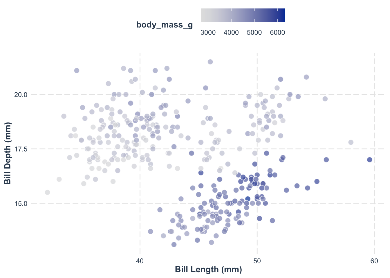
Check more about this topic here.
(Two penguins have a missing body mass or bill measurement, so ggplot2 drops them with a warning, which we hide here.)
A multi-hue sequential palette transitions between several hues (e.g., from yellow through green to blue) while lightness still increases or decreases steadily. The extra hues make small differences easier to tell apart than in a single-hue palette. For example, we can show body mass with the "YlGnBu" palette:
Show the code
library(tidyverse)
library(palmerpenguins)
library(colorspace)
ggplot(penguins, aes(x = bill_length_mm, y = bill_depth_mm, fill = body_mass_g)) +
    geom_point(shape = 21, color = "white", alpha = 0.7, size = 3) +
    scale_fill_continuous_sequential(palette = "YlGnBu") +
    labs(x = "Bill Length (mm)", y = "Bill Depth (mm)") +
    jtools::theme_nice() +
    theme(legend.position = "top")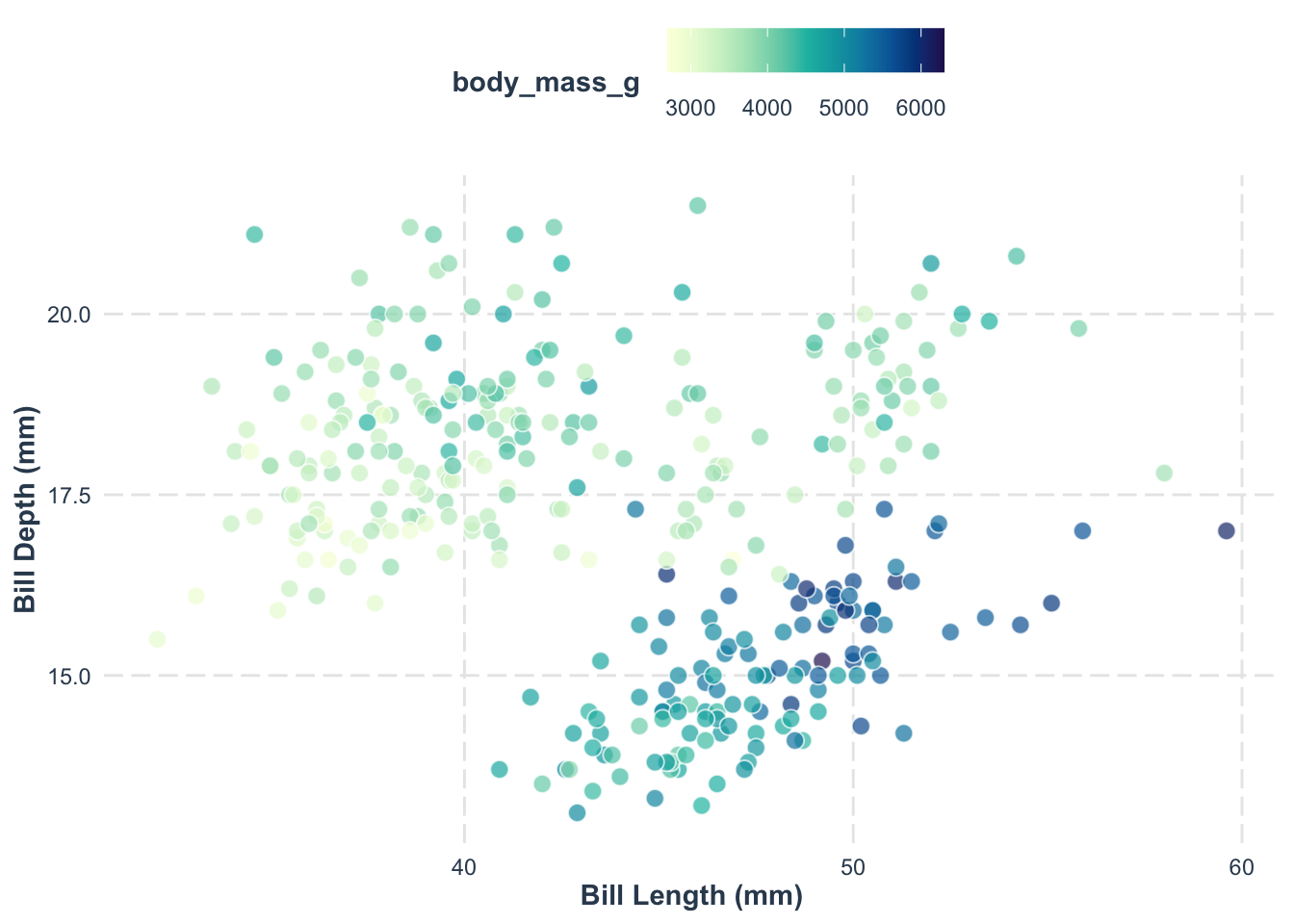
Sometimes you want one color scale to carry two variables. For example, we can use the hue to show the species, and then the lightness within each hue to show the body mass. This needs one single-hue sequential scale per species, which the ggnewscale package makes possible by allowing several fill scales in one plot.
Show the code
library(tidyverse)
library(palmerpenguins)
library(colorspace)
library(ggnewscale)
ggplot(penguins, aes(x = bill_length_mm, y = bill_depth_mm)) +
    geom_point(
        data = filter(penguins, species == "Chinstrap"),
        aes(fill = body_mass_g),
        shape = 21, color = "white", alpha = 0.8, size = 3
    ) +
    scale_fill_continuous_sequential(palette = "Purples 3", name = "Chinstrap") +
    ggnewscale::new_scale_fill() +
    geom_point(
        data = filter(penguins, species == "Adelie"),
        aes(fill = body_mass_g),
        shape = 21, color = "white", alpha = 0.8, size = 3
    ) +
    scale_fill_continuous_sequential(palette = "Blues 3", name = "Adelie") +
    ggnewscale::new_scale_fill() +
    geom_point(
        data = filter(penguins, species == "Gentoo"),
        aes(fill = body_mass_g),
        shape = 21, color = "white", alpha = 0.8, size = 3
    ) +
    scale_fill_continuous_sequential(palette = "Greens 3", name = "Gentoo") +
    labs(x = "Bill Length (mm)", y = "Bill Depth (mm)") +
    jtools::theme_nice() +
    theme(legend.position = "top")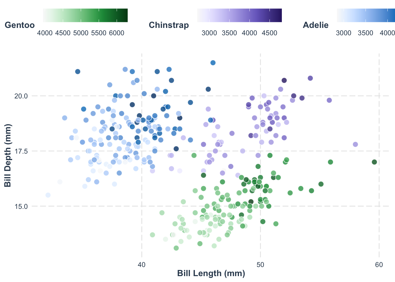
Use two contrasting hues that meet in a neutral middle value. This is ideal when your data diverges around a critical midpoint (e.g., zero).
For example, we want to show whether the penguins are above or below the average body mass, using standardized body mass (z-score), where 0 is the average.
Show the code
library(tidyverse)
library(palmerpenguins)
library(colorspace)

penguins |>
    mutate(body_mass_g = (body_mass_g - mean(body_mass_g, na.rm = TRUE))/sd(body_mass_g, na.rm = TRUE)) |>
    ggplot(aes(x = bill_length_mm, y = bill_depth_mm, fill = body_mass_g)) +
    geom_point(alpha = 0.8, size = 3, shape = 21, color = "white") +
    scale_fill_continuous_diverging(name = "Standardized Body Mass") +
    labs(x = "Bill Length (mm)", y = "Bill Depth (mm)") +
    jtools::theme_nice() +
    theme(legend.position = "top")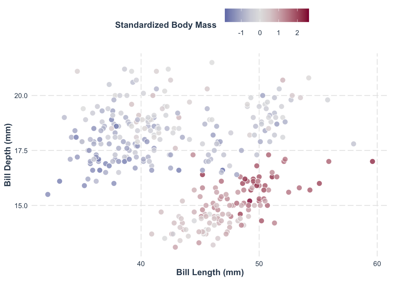
16.1.2 Reduce Chroma
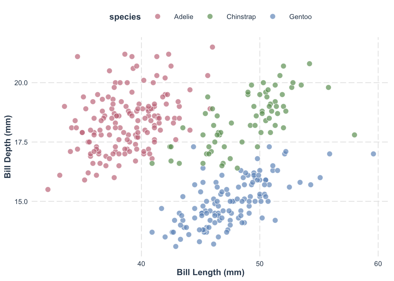
Chroma is the “colorfulness” (saturation) of a color. Highly saturated colors are visually loud, so using them everywhere makes a figure tiring and makes it hard to see which elements matter. Prefer muted, lower-chroma colors for most of the plot and save vivid colors for the elements you want to highlight. See this post by Claus Wilke for more.
Show the code
library(tidyverse)
library(palmerpenguins)
library(colorspace)
ggplot(penguins, aes(x = bill_length_mm, y = bill_depth_mm, fill = species)) +
geom_point(shape = 21, color = "white", alpha = 0.7, size = 3) +
scale_fill_manual(values = desaturate(qualitative_hcl(3, c = 100), amount = 0.5)) +
labs(x = "Bill Length (mm)", y = "Bill Depth (mm)") +
jtools::theme_nice() +
theme(legend.position = "top")- 1
-
desaturate()lowers the chroma of the palette; compare with the defaultscale_fill_discrete_qualitative()above.
16.1.3 Be aware of color-vision deficiency
Additionally, whenever possible, always verify that your plot is color-blind friendly. Many modern palettes are designed to be distinguishable for viewers with common forms of color vision deficiency. If you are interested, you can read more here.
16.2 My Go-To Solution: The colorspace Package
Based on these considerations, my preferred tool is the colorspace package. It provides a unified and flexible interface to generate color palettes tailored to the type of data you are visualizing.
For example, consider the following code that uses colorspace to create a scatterplot of penguins data:
library(tidyverse)
library(colorspace)
library(palmerpenguins)

penguins |>
    ggplot(aes(x = bill_length_mm, y = bill_depth_mm, color = species)) +
    geom_point() +
    scale_color_discrete_qualitative() +
    jtools::theme_nice()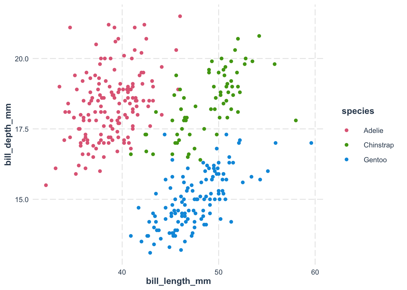
The color scale function–scale_color_discrete_qualitative()–is part of the colorspace package. Its naming convention follows the structure:
scale_<aesthetic>_<datatype>_<colorscale>()<aesthetic>: The visual attribute (e.g., color or fill).<datatype>: The type of data being mapped (discrete,continuous, orbinned).<colorscale>: The palette type (qualitative,sequential, ordiverging).
For example, scale_fill_continuous_sequential() maps continuous data to a sequential palette, and scale_color_discrete_qualitative() maps a discrete variable to a qualitative palette.
DON’T use the rainbow color palette.
Although visually striking, rainbow palettes can distort data interpretation. Their perceived brightness is uneven, so false “edges” appear where none exist in the data. They have no natural low-to-high order, and they are hard to read for viewers with color-vision deficiency. Compare scale_fill_continuous_sequential() with scale_fill_gradientn(colors = rainbow(7)) on the same data.
Use the
viridis palettes for color-vision-deficiency-safe scales.
Another popular package is viridis package, which offers excellent color palettes. As an example,
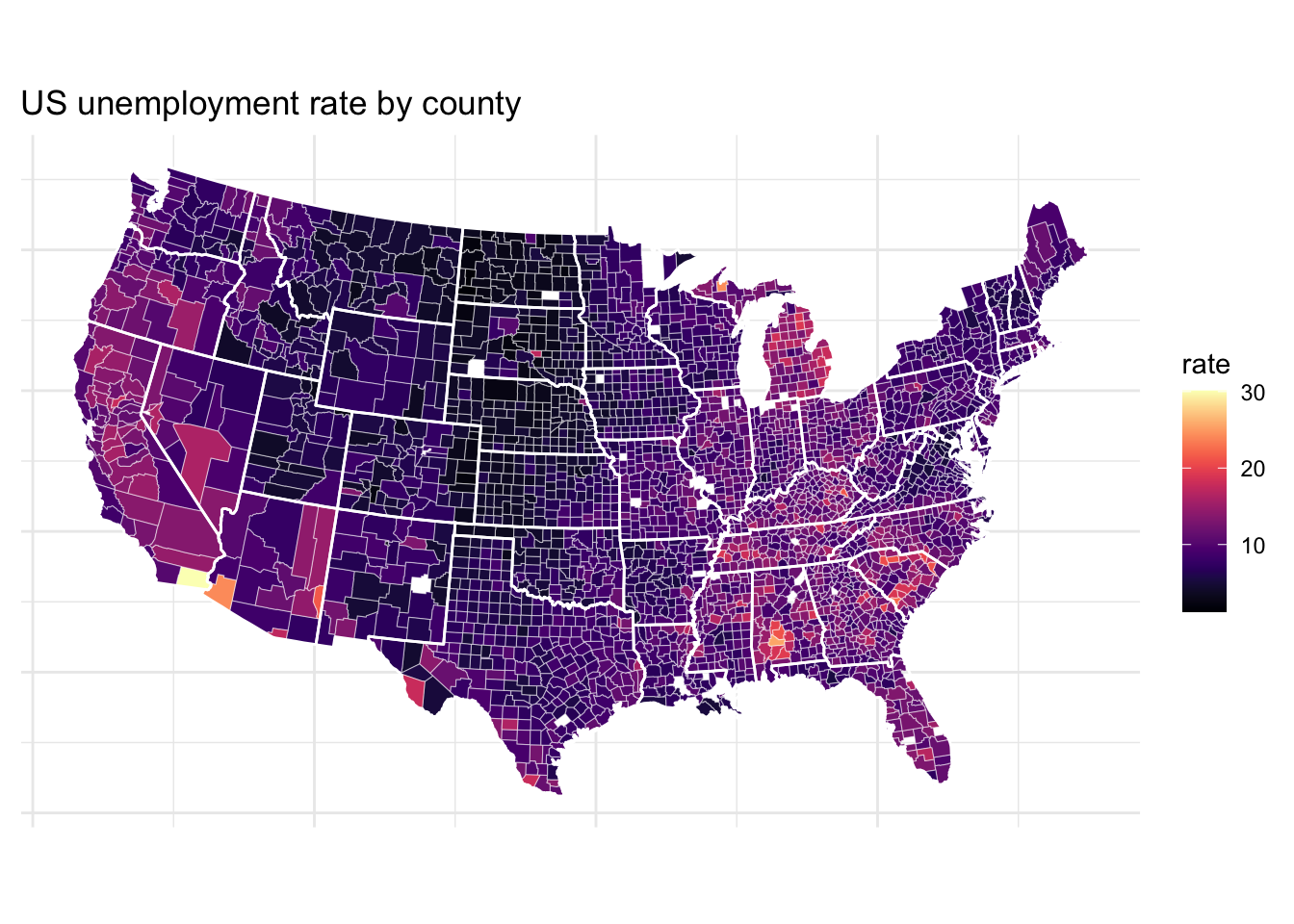
viridis palettes are designed to be perceptually uniform and readable for most forms of color-vision deficiency, which is the main reason to use them. ggplot2 ships scale_*_viridis_d(), scale_*_viridis_c(), and scale_*_viridis_b() for discrete, continuous, and binned data. It is less flexible than colorspace, though, because it offers no diverging or qualitative palette families.
16.3 Additional Useful Resources
- color-palette-finder: An interactive tool to help you choose the right color palette for your visualization.
- 配色事典: A visually rich resource with a wide range of palettes. I like having a physical copy when choosing colors.
- Traditional colors: A collection of traditional colors used in China and Japan. There are many other color palettes available online from different cultures. Try to explore them!
- ColorPick Eye Dropper: A tool in Chrome that allows you to pick colors from any image and convert them to HEX code.