3 Basic Data Structure

Class Objectives

Understand vector and tibble in R
Get comfortable with R’s common data types

A data structure is an orderly, efficient way to store and retrieve data. While it may feel a bit abstract if you’re new to coding, think of these structures as the “nouns” in your programming language (with data wrangling serving as the “verbs”).

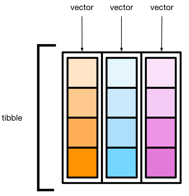
R has provided many data structures. Fortunately, nine times out of ten, you’ll only need to worry about two: vector and tibble.

3.1 Vector

A vector is a one-dimensional array—like a row of seats in a movie theater that only allows one type of audience member, be they numeric, character, or logical. We create them with the c() function. For example:

numbers <- c(1, 2, 3, 4, 5)
numbers

1: Create a vector of numbers from 1 to 5.
2: Display the numbers vector.

[1] 1 2 3 4 5

What does c() stand for

c() means “combine.” Yes, it’s a slightly cryptic name for what you’ll soon be typing all the time, but you’ll get used to it.

Vectors form the backbone of R scripts. They’re how you can store the number of penguins wandering around Antarctica, keep track of class attendance, or tally cars on the highway. A key detail: everything in a vector must share the same type. Some common types are:

numeric (like 3.14 or 42)
character (like “Hello” or “World”)
logical (TRUE or FALSE)
factor (categorical data)

Below, we make a few different vectors to illustrate these types:

numbers <- c(1.1, 2.2, 3.3, 4.4, 5.5)
characters <- c("a", "b", "c")
logicals <- c(TRUE, FALSE, TRUE)
factors <- factor(c("a", "b", "c"))

1: Create a vector of numbers from 1 to 5.
2: Create a vector of characters.
3: Create a vector of logicals.
4: Create a vector of factors.

Be aware of data types

R automatically assigns the data type for each vector, which can save time but also lead to (unwanted) surprises. For instance, sometimes 1 appears as a character rather than a number—something that can introduce annoying bugs. Avoid headaches by checking data types with class(). For example:

class(numbers)

[1] "numeric"

A horror story (not in R but in Excel) is that the auto-convert feature messes up gene names like SEPT4 to 4-Sept (datatype from character to datetime). This has affected a ton of genetic papers. So, always be aware of the data types!

We can also extract data from a vector using the square brackets []. For example:

numbers[1]
characters[2]

1: Extract the first element from the numbers vector.
2: Extract the second element from the characters vector.

[1] 1.1
[1] "b"

Note that the index starts from 1, not 0. This is a common source of confusion for those coming from languages like Python or C. I personally prefer the 1-based index, as this is more intuitive.

Exercise

Create a vector of numbers from -1 to -3, and then extract the second element.

Exercise
Solution

Create a vector of characters with your name and surname.

Exercise

Create a vector of logicals by flipping a coin three times.

Exercise

3.2 Tibble

A tibble (brought to you by the tidyverse) is essentially a set of vectors bound together in columns—like a multi-row, multi-column theater, where each column houses a single data type.

As a simple xample,

library(tidyverse)
tibble(
    x = c(1, 2, 3),
    y = c("a", "b", "c"),
    z = c(TRUE, FALSE, TRUE)
)

1: Load the tidyverse package, as tibble is from it.
2: Create a tibble.
3: Create the first column as a vector of numbers from 1 to 3.
4: Create the second column as a vector of characters.
5: Create the third column as a vector of logicals.
6: Always remember to close the function with a parenthesis.

Another way to write tibble

There is another equivalent way of writing it rowwisely. For example,:

tribble(
  ~x, ~y,
  1, "a",
  2, "b", 
  3, "c"
)

1: Create a tibble rowwisely (note the function name is different from tibble).
2: Define the column names.
3: Define the first row.

This is perfect when typing in smaller datasets by hand.

Tibbles come with plenty of benefits over base R’s classic data frame—particularly in how they track and preserve data types. You’ll notice each column explicitly labeled as dbl (double) or chr (character), which can save you from those frustrating mysteries where your numeric data gets disguised as text.

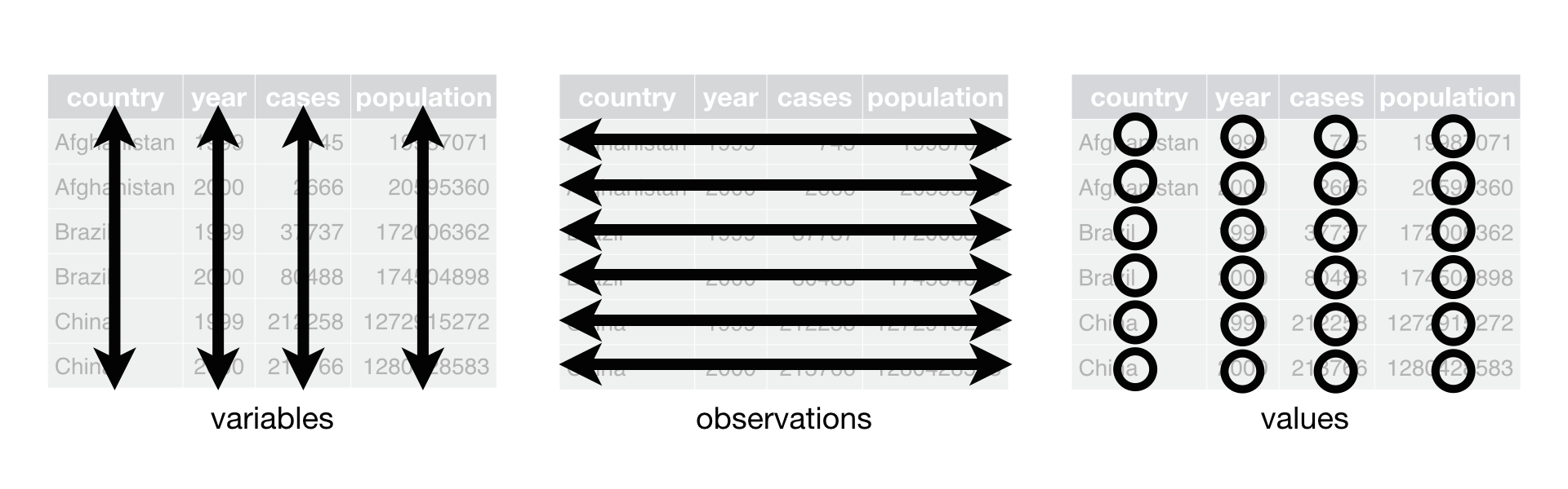
Tibbles also enforce a neat and consistent data layout, called Tidy Data, which is a godsend when you’re dealing with other people’s messy spreadsheets. Quoting from Hadley Wickham (link):

Tidy datasets are easy to manipulate, model and visualize, and have a specific structure: each variable is a column, each observation is a row, and each type of observational unit is a table.

From https://r4ds.hadley.nz/data-tidy.html

We will learn more about working with tibble more in the next sections, but for now, let’s move on to our example dataset.

Exercise

Create a tibble with the following columns:

name with your name and surname
age with your age
is_student with a logical value

Exercise
Solution

3.3 Our example dataset: `penguins`

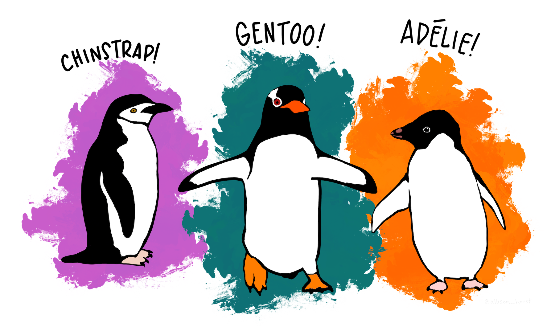
We’ll soon learn how to import data (another comedic ordeal in itself), but for now, let’s borrow the penguins dataset from the palmerpenguins package. It covers three penguin species—Adelie, Chinstrap, and Gentoo—and gives us some useful variables to play with. Who doesn’t love penguins?

First things first, let us load the penguins dataset.

# install.packages("palmerpenguins")
library(palmerpenguins)
data(package = "palmerpenguins")

1: If you have not installed the palmerpenguins package, you can install it by uncommenting this line.
2: Load the palmerpenguins package.
3: Load the penguins dataset.

3.4 Take a Look at your Data

As a first rule, always, always take a look at your data. The simplest way is simply to print it out:

penguins

1: Display the penguins dataset.

This prints about the first couple rows of the dataset (another reason to love tibble over data frame in base R).

You may notice some NA values in the dataset. These are missing values, which are common in real-world datasets. We’ll learn how to handle them later.

3.5 A more structured view

If you’d like a better view of your dataset, try the skim() function from the skimr package:

pacman::p_load(skimr)
skim(penguins)

1: Load the skimr package.
2: Display the summary of the penguins dataset.

Data summary
Name	penguins
Number of rows	344
Number of columns	8
_______________________
Column type frequency:
factor	3
numeric	5
________________________
Group variables	None

Variable type: factor

skim_variable	n_missing	complete_rate	ordered	n_unique	top_counts
species	0	1.00	FALSE	3	Ade: 152, Gen: 124, Chi: 68
island	0	1.00	FALSE	3	Bis: 168, Dre: 124, Tor: 52
sex	11	0.97	FALSE	2	mal: 168, fem: 165

Variable type: numeric

skim_variable	n_missing	complete_rate	mean	sd	p0	p25	p50	p75	p100	hist
bill_length_mm	2	0.99	43.92	5.46	32.1	39.23	44.45	48.5	59.6	▃▇▇▆▁
bill_depth_mm	2	0.99	17.15	1.97	13.1	15.60	17.30	18.7	21.5	▅▅▇▇▂
flipper_length_mm	2	0.99	200.92	14.06	172.0	190.00	197.00	213.0	231.0	▂▇▃▅▂
body_mass_g	2	0.99	4201.75	801.95	2700.0	3550.00	4050.00	4750.0	6300.0	▃▇▆▃▂
year	0	1.00	2008.03	0.82	2007.0	2007.00	2008.00	2009.0	2009.0	▇▁▇▁▇

Think of skim() as your quick backstage pass, telling you how many rows, columns, missing values, and data types you’re dealing with. Trust me, a few seconds spent peeking at your data can save hours of confusion down the line.

Exercise

iris is a widely-used dataset of plant traits. It is a default dataset in R. Take a look at the iris dataset using the skim() function.

Exercise
Solution

3.1 Vector

Exercise

3.2 Tibble

Exercise

3.3 Our example dataset: penguins

3.4 Take a Look at your Data

3.5 A more structured view

Exercise

3.3 Our example dataset: `penguins`