pak::pak(c("tidyverse", "janitor", "mgcv", "gghighlight", "plotly", "ggalt", "zoo", "ggstream", "ggh4x", "ggrepel", "MetBrewer", "hrbrthemes"))13 Visualizing Trends
Class Objectives:
- Trend of a single variable
- Smoothed trends
- Trend of multiple groups
Packages for this chapter
If you haven’t installed the following packages, run this code:
Trend plots show how a measured quantity changes along an ordered variable, usually time. Start with the observed values, then decide whether a line, a summary, or a smoother helps answer your question. Connecting observations implies an order; it is not appropriate for unrelated categories.
As in Chapter 12, load tidyverse to use its functions directly, and use package::function() for other packages, including janitor::clean_names() to clean column names. We use a different theme this time, with a generic font so the examples do not require extra font installation.
library(tidyverse)
theme_set(hrbrthemes::theme_ipsum(base_family = "sans"))- 1
- Set the theme for the plots.
13.1 A Basic Trend Plot
We use economics, a historical monthly dataset. Its unemploy column counts unemployed people in thousands; it is not an unemployment rate. First, clean the names and put the observations in chronological order. The names are already tidy here, but we keep the same preparation workflow as in the data-import chapter.
economics_monthly <- economics |>
    janitor::clean_names() |>
    arrange(date)

economics_recent <- economics_monthly |>
    filter(year(date) > 2000)
For the first examples, select January from each year to make the individual observations easy to see. These are January snapshots, not annual averages.
economics_recent |>
    filter(month(date) == 1) |>
    ggplot(aes(x = date, y = unemploy)) +
    labs(x = "Year", y = "Unemployed people (thousands)") +
    geom_point(color = "white", fill = "#0072B2", shape = 21, size = 2)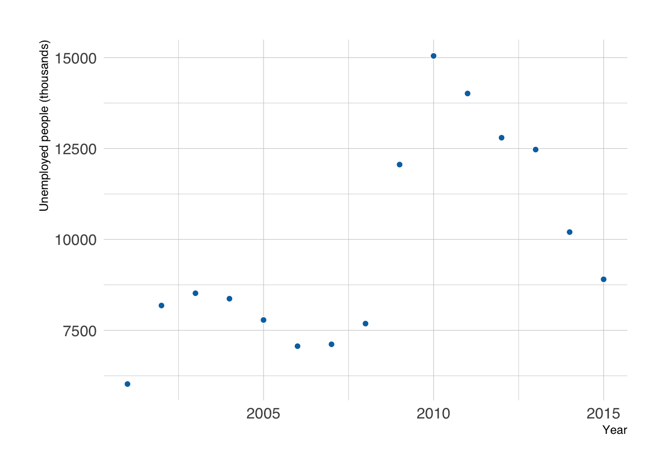
The date stays on a continuous time axis, so the distance between points represents elapsed time.
The points show individual measurements. Connecting them makes changes between successive observations easier to follow.
Connect the dots with a line to reveal the trend. This is easy to do with geom_line().
economics_recent |>
    filter(month(date) == 1) |>
    ggplot(aes(x = date, y = unemploy)) +
    labs(x = "Year", y = "Unemployed people (thousands)") +
    geom_line(linewidth = 1, color = "#0072B2") +
    geom_point(color = "white", fill = "#0072B2", shape = 21, size = 4)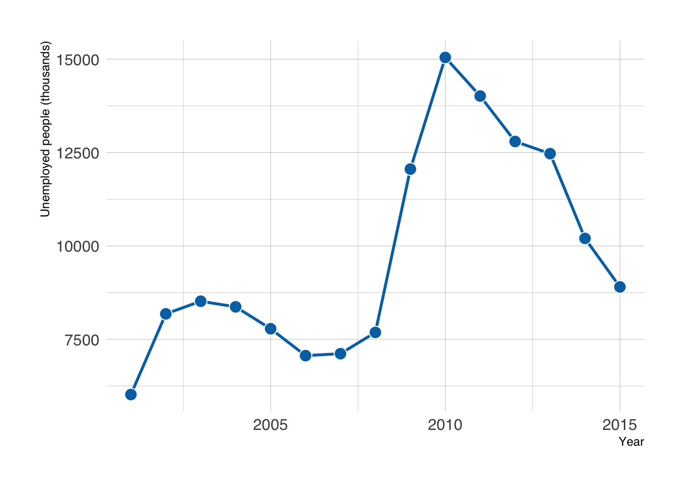
A white border helps the points stand out against the line. geom_line() connects points in x order; geom_path() follows the row order instead. Neither one establishes what happened between observations. If a scheduled observation is missing, keep its date with an NA value to show a gap rather than silently connecting across it.
An interpolating spline draws a curved connection between observations. ggalt::geom_xspline() provides this option. The curve is a drawing choice, not a fitted statistical model: it can suggest peaks or dips between dates where no measurement was taken. Prefer straight segments when those extra shapes could mislead.
economics_recent |>
    filter(month(date) == 1) |>
    ggplot(aes(x = date, y = unemploy)) +
    labs(x = "Year", y = "Unemployed people (thousands)") +
    ggalt::geom_xspline(color = "#0072B2") +
    geom_point(color = "white", fill = "#0072B2", shape = 21, size = 4)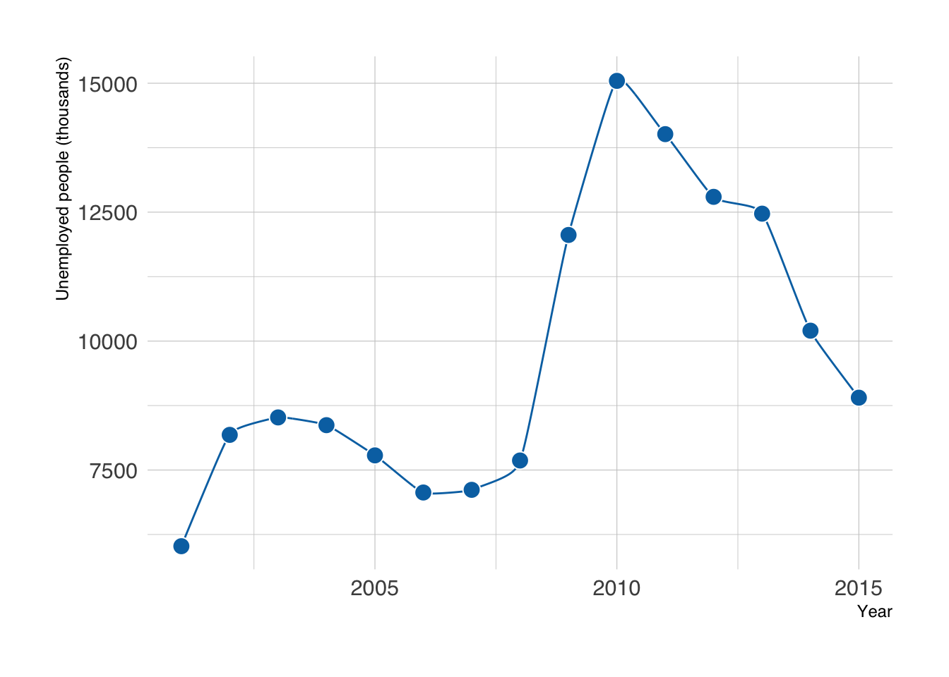
An area plot emphasizes the magnitude of a nonnegative quantity by filling the space between the line and zero. Use it when zero is a meaningful baseline, and keep that baseline visible. Draw the area first so it sits behind the line and points.
economics_recent |>
    filter(month(date) == 1) |>
    ggplot(aes(x = date, y = unemploy)) +
    labs(x = "Year", y = "Unemployed people (thousands)") +
    geom_area(fill = "#0072B2", alpha = 0.2) +
    geom_line(linewidth = 1, color = "#0072B2") +
    geom_point(color = "white", fill = "#0072B2", shape = 21, size = 4)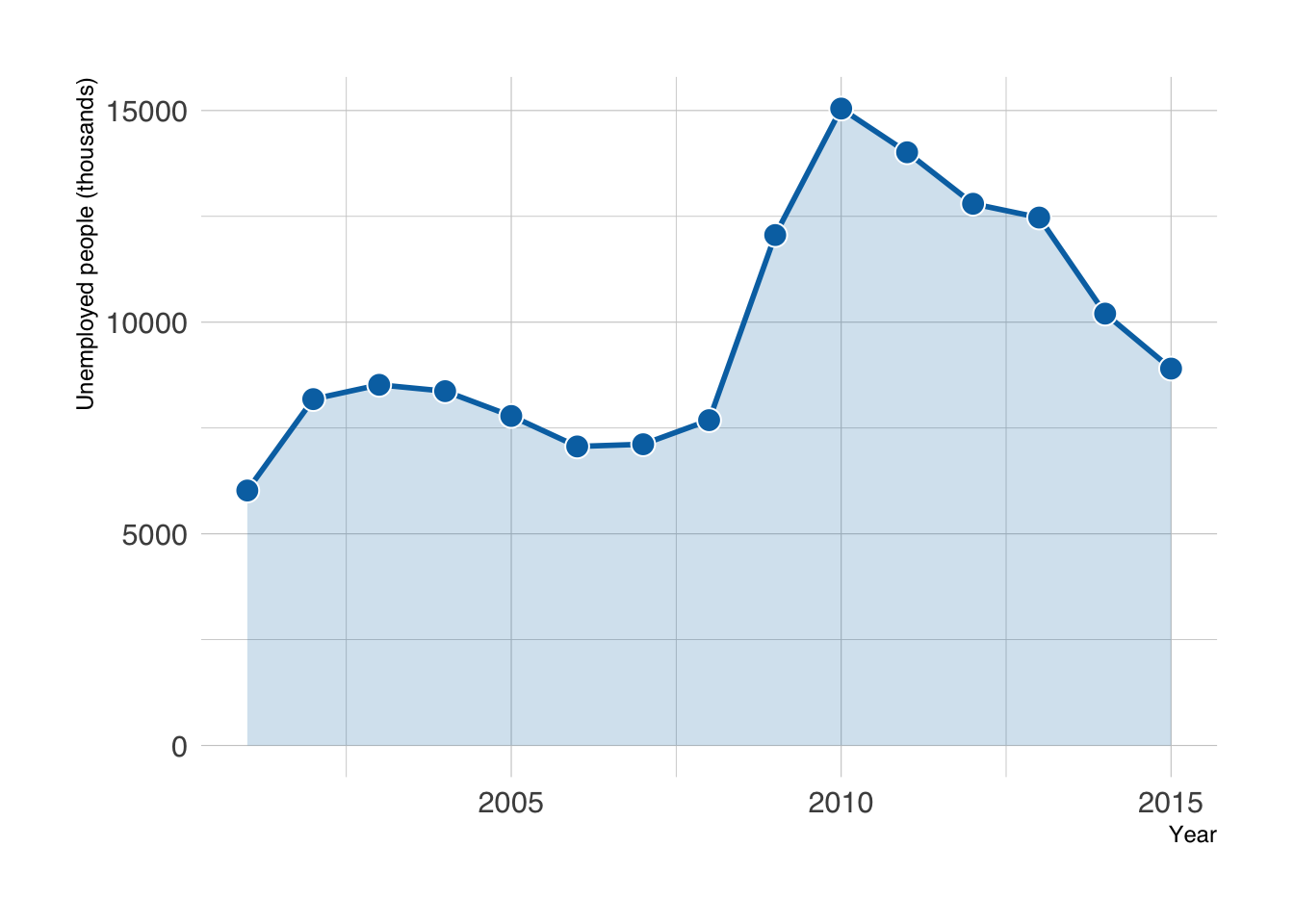
13.2 Dealing with Many Points
With monthly observations, large point symbols can crowd the line. Smaller points or a line alone may be enough; smoothing is useful when the question concerns changes over a longer timescale.
economics_recent |>
    ggplot(aes(x = date, y = unemploy)) +
    labs(x = "Year", y = "Unemployed people (thousands)") +
    geom_line(color = "#0072B2") +
    geom_point(color = "white", fill = "#0072B2", shape = 21, size = 3)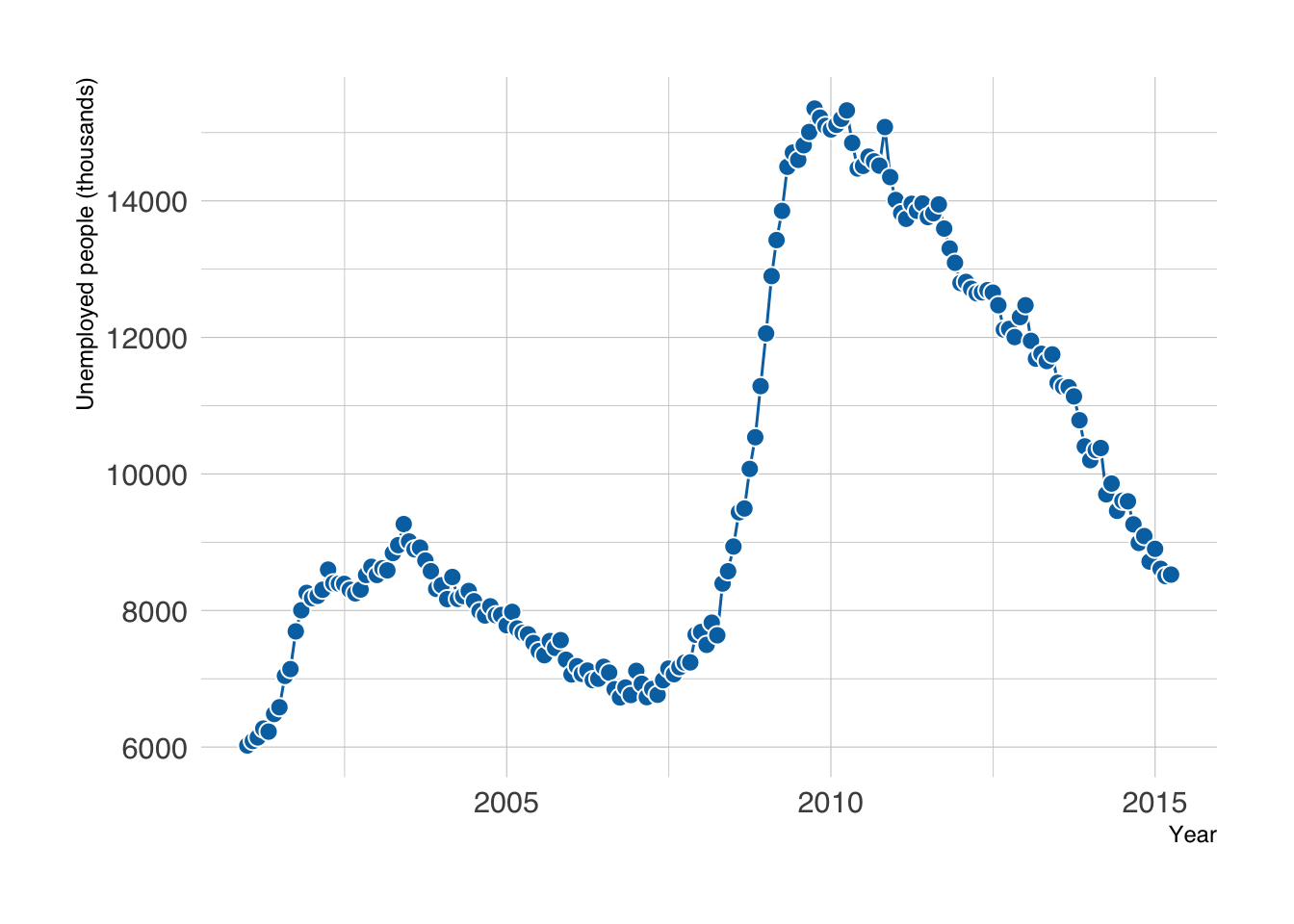
Below are some alternatives to consider, from the least to the most modelling.
The simplest fix is to remove clutter before adding anything: drop the points and let the line carry the trend.
economics_recent |>
    ggplot(aes(x = date, y = unemploy)) +
    labs(x = "Year", y = "Unemployed people (thousands)") +
    geom_line(color = "#0072B2")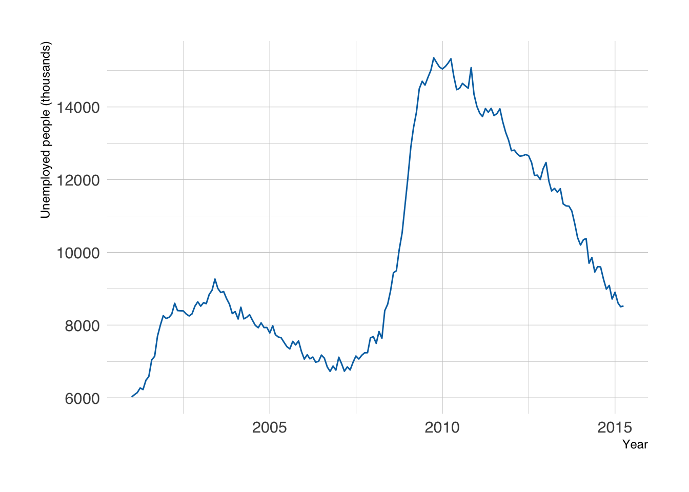
If month-to-month wiggles still distract from the question, summarize the data with one of the next approaches.
Aggregating replaces many observations with one summary per coarser time step, such as one mean per year. No model is involved, so the result is easy to explain: “the average monthly unemployment in each year.”
economics_recent |>
mutate(year = year(date)) |>
filter(n() == 12, .by = year) |>
summarise(unemploy = mean(unemploy), .by = year) |>
ggplot(aes(x = year, y = unemploy)) +
labs(x = "Year", y = "Mean unemployed people (thousands)") +
geom_line(color = "#0072B2") +
geom_point(color = "white", fill = "#0072B2", shape = 21, size = 3)- 1
- Extract the year from each date.
- 2
- Keep only complete years. The data end in April 2015, and a mean of four months is not comparable with a mean of twelve.
- 3
-
Collapse each year to its mean. Use
median()instead if a few extreme months should not dominate.
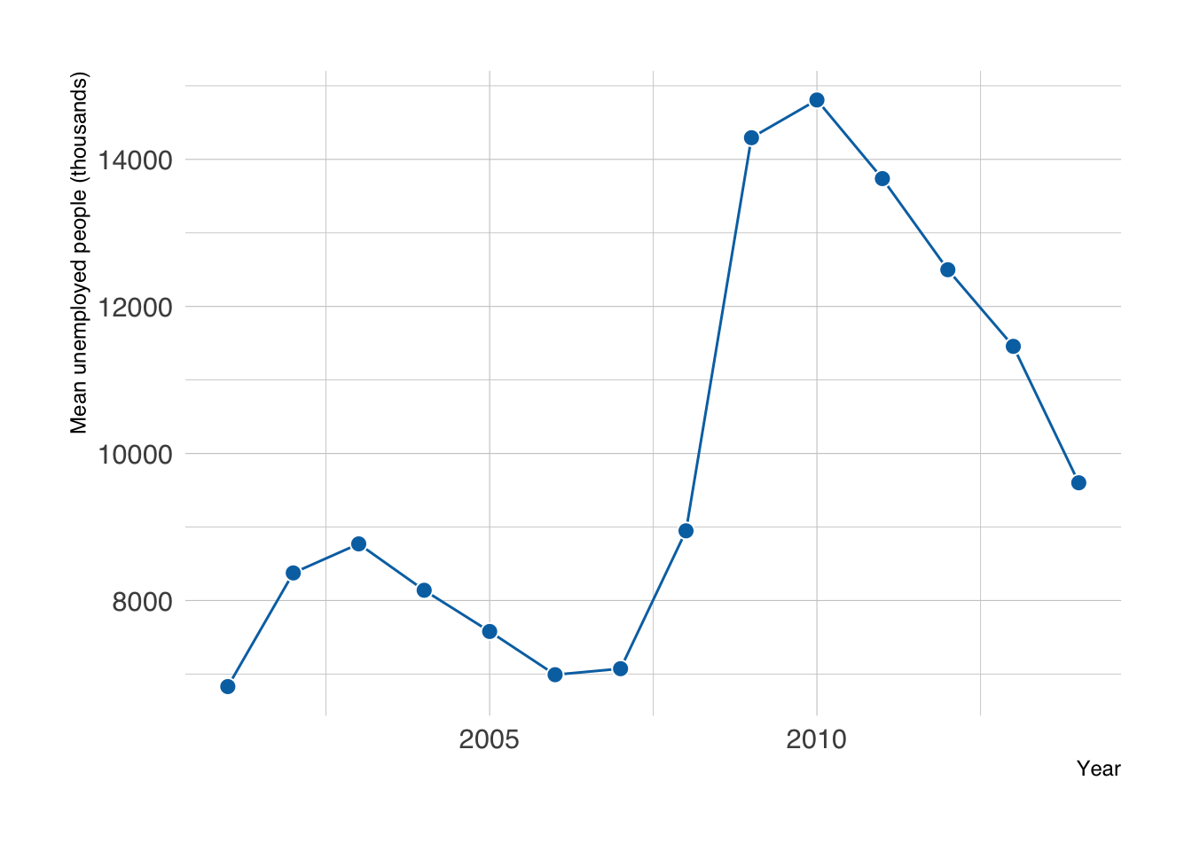
Aggregation also hides change within each period: a recession that starts in October looks like a small rise in that year’s mean.
A moving average replaces each observation with the mean of a nearby window. A longer window removes more short-term variation but can hide brief events and delay turning points.
Use zoo::rollmean() on the chronologically ordered monthly data. Here, 12 rows represent 12 consecutive months. With irregular sampling or missing months, a 12-row window is not necessarily a year: regularize the dates and decide how to handle missing measurements first. Compute the averages before selecting the display period so earlier observations remain available to its first windows.
economics_averages <- economics_monthly |>
mutate(unemploy_avg_year = zoo::rollmean(unemploy, k = 12, fill = NA, align = "right")) |>
mutate(unemploy_avg_2years = zoo::rollmean(unemploy, k = 24, fill = NA, align = "right"))
economics_averages |>
filter(year(date) > 2000) |>
ggplot(aes(x = date, y = unemploy)) +
labs(x = "Year", y = "Unemployed people (thousands)") +
geom_line(aes(color = 'line')) +
geom_line(aes(y = unemploy_avg_year, color = 'year'), linewidth = 1) +
geom_line(aes(y = unemploy_avg_2years, color = '2 years'), linewidth = 1) +
scale_color_manual(
values = c(`line` = "grey60", `year` = "#d55e00", `2 years` = "#009E73"),
breaks = c("year", "2 years", "line"),
labels = c("Trailing 12 months", "Trailing 24 months", "Monthly observations"),
name = NULL
) +
theme(legend.position = 'top')- 1
-
Calculate the moving average of the current and previous 11 months (
align = "right"; the defaultalign = "center"would center the window on each month instead). - 2
- Calculate the moving average of the current and previous 23 months.
- 3
- Add the moving average for the last 12 months to the plot.
- 4
- Add the moving average for the last 24 months to the plot.
- 5
- Customize the color legend.
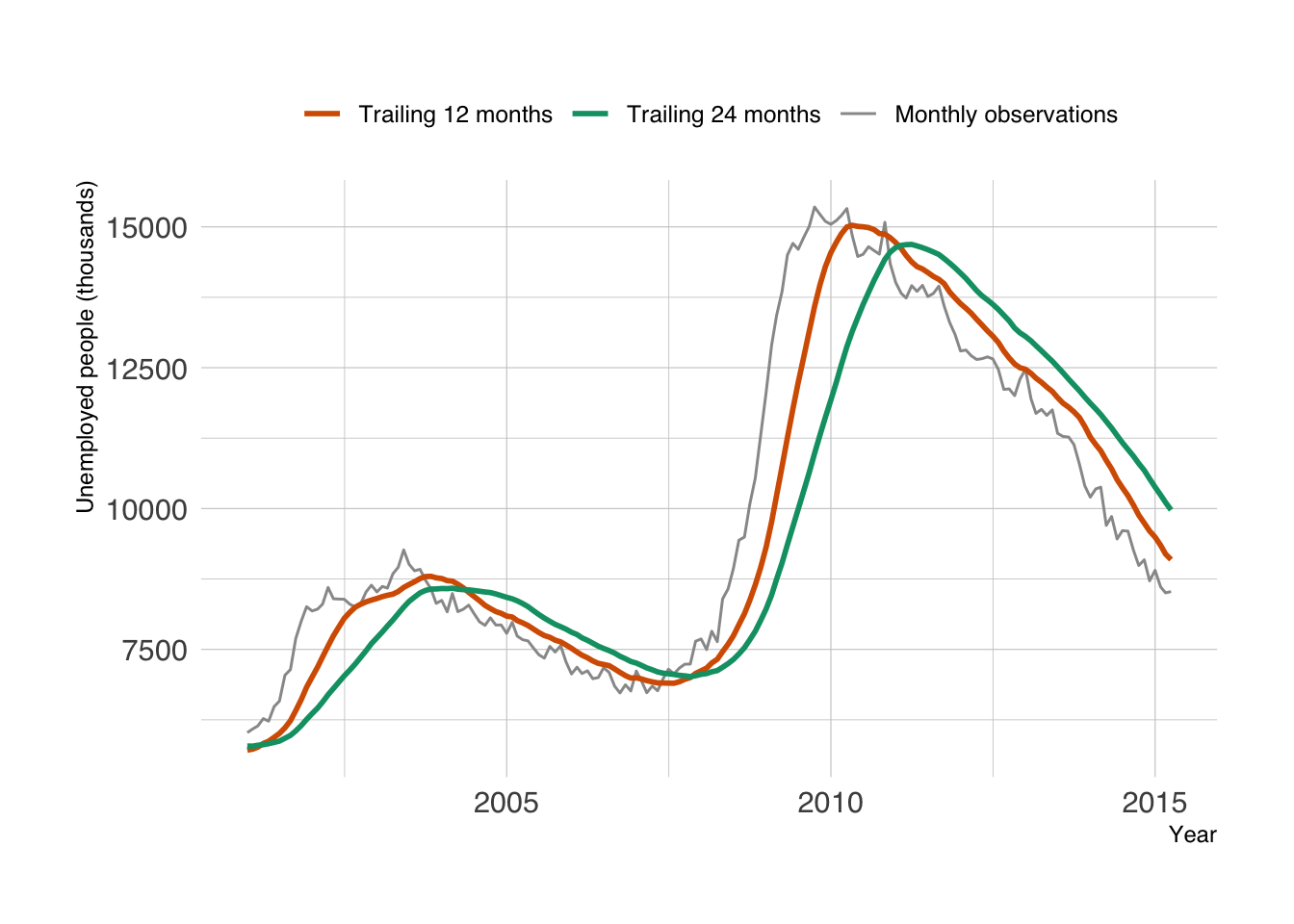
The first 11 (or 23) observations in the full series have no complete window, so their averages are NA. They precede the displayed period here. A trailing average uses the current and previous observations; a centered average also uses future observations relative to its plotted date.
Alternatively, you can add a regression smoother to highlight the trend. We have already used the linear regression smoother with geom_smooth(method = "lm") in Chapter 6. It is easy to use other nonlinear methods.
economics_recent |>
ggplot(aes(x = date, y = unemploy)) +
labs(x = "Year", y = "Unemployed people (thousands)") +
geom_point(color = "white", fill = "grey60", shape = 21, size = 3) +
geom_smooth(method = "loess", span = 0.3, se = FALSE)- 1
-
Fit a LOESS (local regression) smoother.
spanis the fraction of the data used for each local fit: smaller values follow the data more closely, larger values give a smoother curve. Try 0.1 and 0.75 to see the difference.
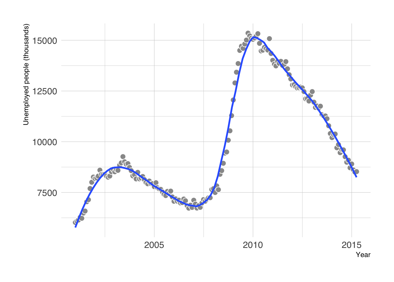
Specify the smoothing method and keep the observations visible. We set se = FALSE because this is a descriptive trend: a reliable uncertainty interval for time-series data needs to account for dependence between nearby observations. The default smoother ribbon is not a prediction interval or a forecast.
Additionally, when handling a lot of data, you can fit the model yourself once (for example with mgcv::gam()) and plot its predictions, instead of letting ggplot2 refit the smoother every time you draw the plot.
13.3 Visualizing Trends in Multiple Groups
For multiple groups, use one row per group and time point, and map the group to color or fill. The ggstream::blockbusters dataset summarizes box office by genre and year for a selected sample of top-grossing films. Its units are billions of inflation-adjusted dollars; it does not describe the entire film market.
Some genre–year combinations are absent from this table. For this example, we explicitly interpret an absent combination as zero contribution to the selected blockbuster sample. complete() makes those zeros visible to the plotting functions. For genuinely unknown values in another dataset, leave NA instead; zero is a substantive assumption.
blockbusters <- ggstream::blockbusters |>
janitor::clean_names() |>
complete(year, genre, fill = list(box_office = 0)) |>
arrange(genre, year)
blockbusters |>
ggplot(aes(x = year, y = box_office, color = genre, group = genre)) +
labs(x = "Year", y = "Box office (billions of real dollars)", color = "Genre") +
geom_line()- 1
- Add the absent combinations with zero box office under the assumption stated above.
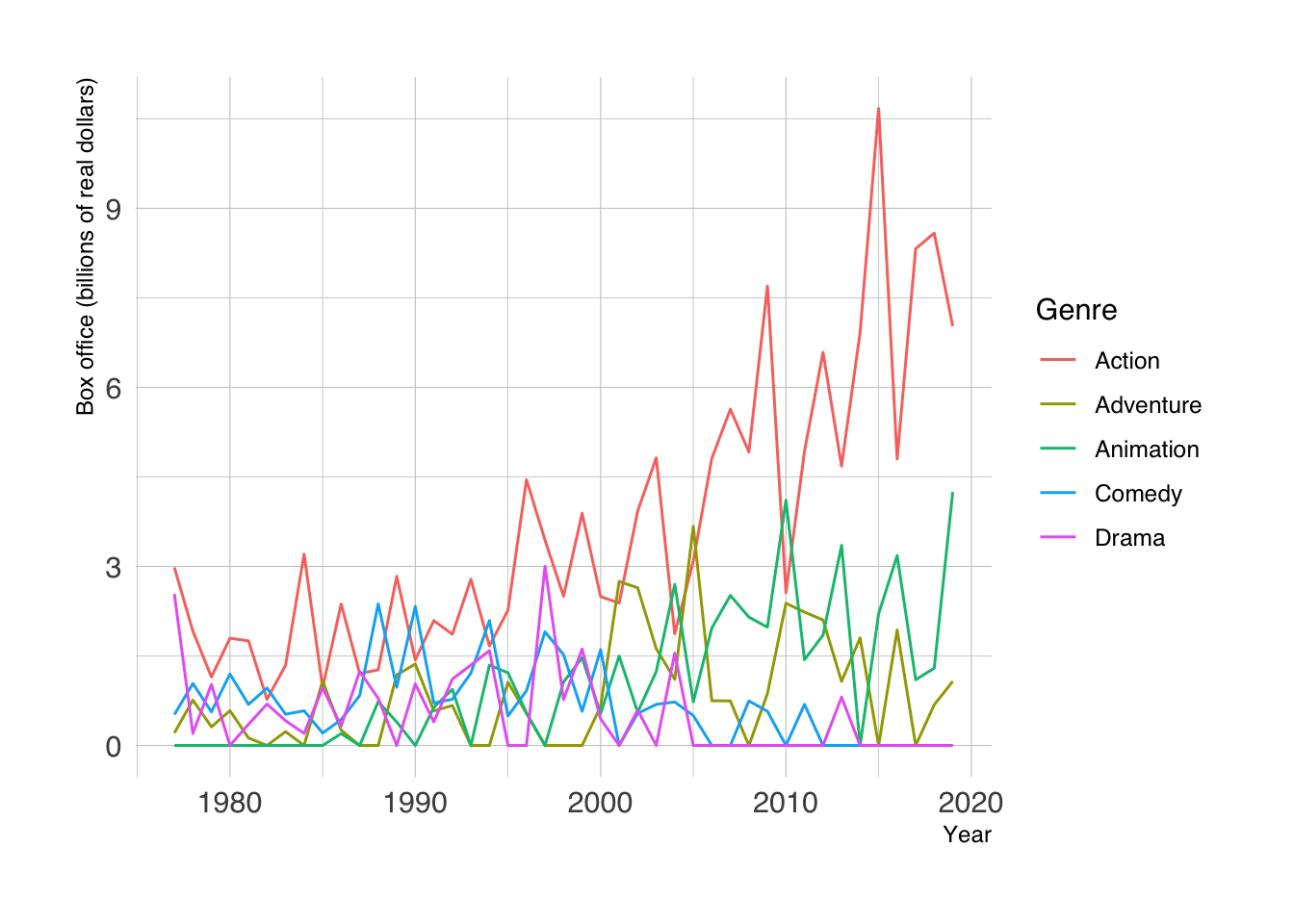
Color distinguishes the groups, but overlapping lines can still hide individual trajectories. Choose the next display based on whether the question is about each group, the total, or relative rank.
We can also use facets to show the trend of each group.
blockbusters |>
    ggplot(aes(x = year, y = box_office, color = genre, group = genre)) +
    labs(x = "Year", y = "Box office (billions of real dollars)", color = "Genre") +
    geom_line(linewidth = .5) +
    facet_wrap(~genre) +
    MetBrewer::scale_color_met_d("Cross") +
    theme(legend.position = 'none')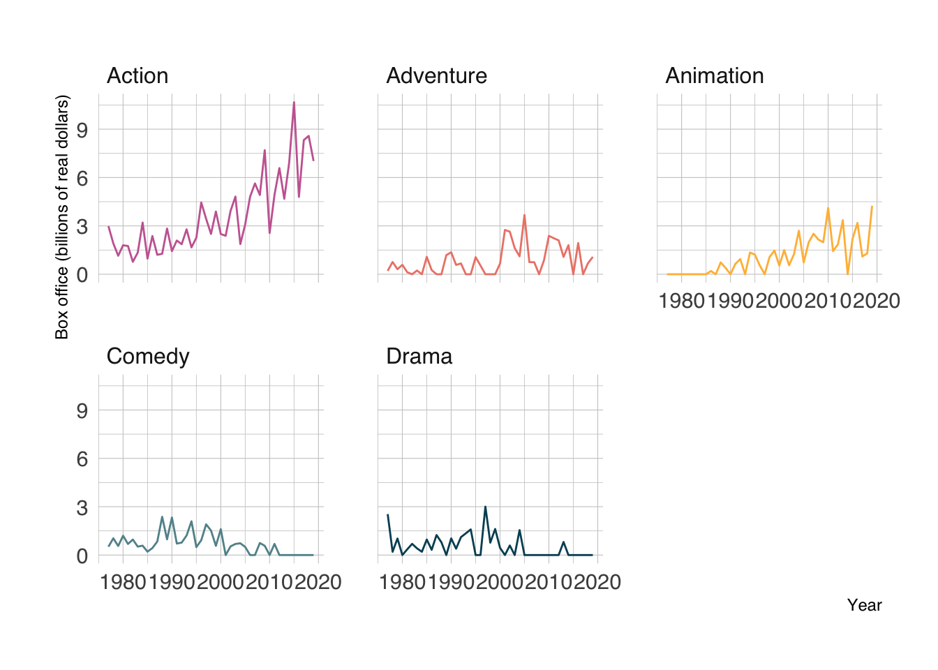
Shared axis limits let us compare magnitudes across facets. To make the other groups visible as context within each panel, use gghighlight::gghighlight(). Avoid free y scales when absolute differences between groups matter.
blockbusters |>
    ggplot(aes(x = year, y = box_office, color = genre, group = genre)) +
    labs(x = "Year", y = "Box office (billions of real dollars)", color = "Genre") +
    geom_line(linewidth = .5) +
    gghighlight::gghighlight(use_direct_label = FALSE,
                unhighlighted_params = list(colour = "grey85")) +
    facet_wrap(~genre) +
    MetBrewer::scale_color_met_d("Cross") +
    theme(legend.position = 'none')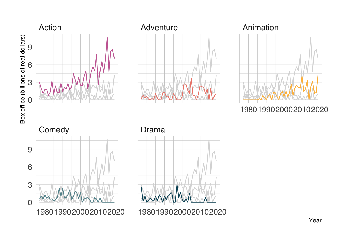
A stacked area plot shows how nonnegative, non-overlapping categories contribute to a total. The upper boundary is the total, and each band’s thickness is its category’s contribution. Here, the total refers only to the genres and films in this dataset.
blockbusters |>
    ggplot(aes(x = year, y = box_office, fill = genre)) +
    labs(x = "Year", y = "Box office (billions of real dollars)", fill = "Genre") +
    geom_area() +
    MetBrewer::scale_fill_met_d("Cross")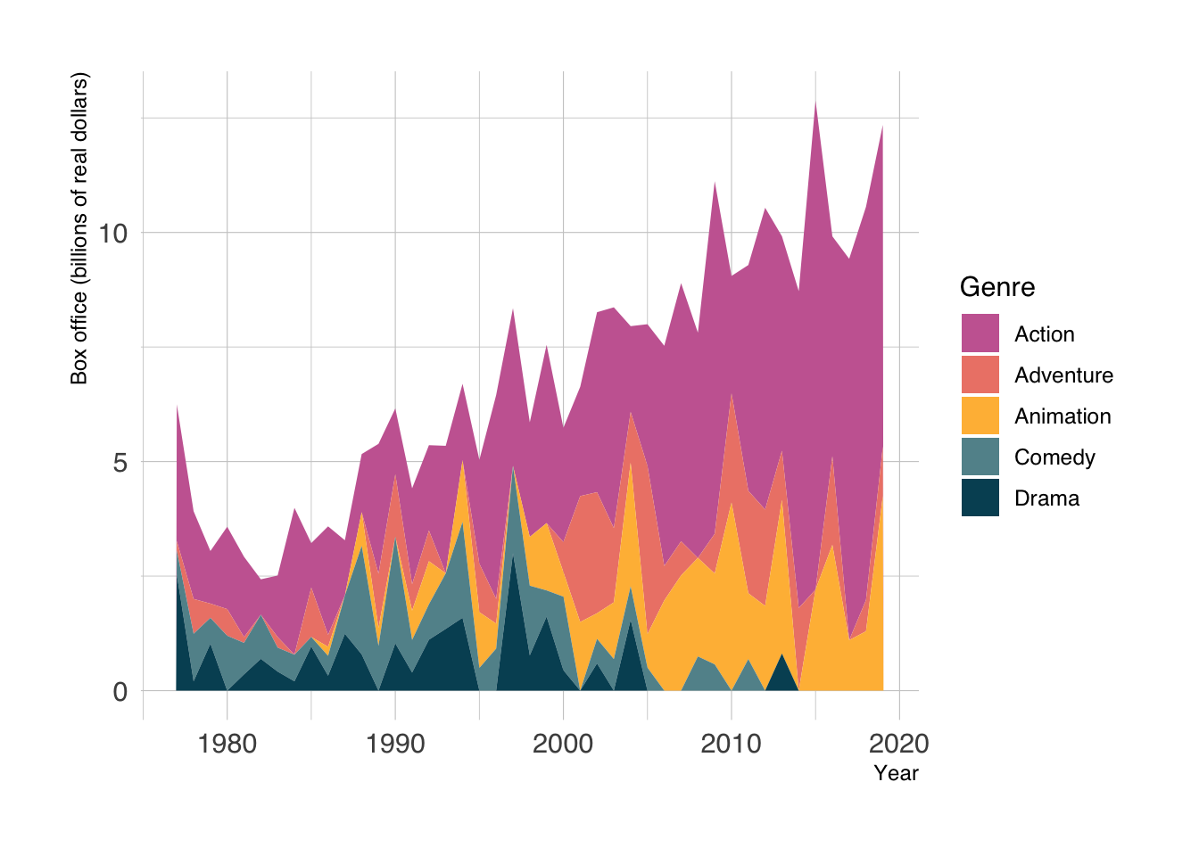
Only the bottom band has a fixed baseline. Comparing changes in the upper bands is harder; use lines or facets when individual trajectories matter more than the total.
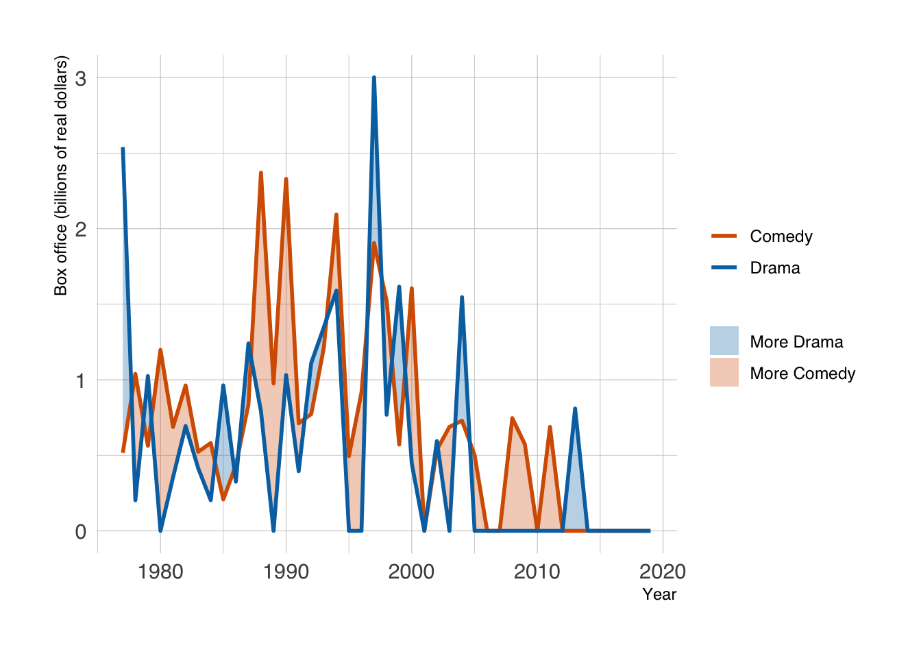
For only two groups, a different display works well: draw both lines and shade the difference between them, colored by which group is higher (ggh4x::stat_difference()).
blockbusters |>
filter(genre %in% c("Comedy", "Drama")) |>
pivot_wider(names_from = genre, values_from = box_office) |>
janitor::clean_names() |>
ggplot(aes(x = year)) +
ggh4x::stat_difference(
aes(ymin = comedy, ymax = drama),
levels = c("More Drama", "More Comedy"), alpha = 0.3
) +
geom_line(aes(y = comedy, color = "Comedy"), linewidth = 1) +
geom_line(aes(y = drama, color = "Drama"), linewidth = 1) +
scale_fill_manual(values = c("More Drama" = "#0072B2", "More Comedy" = "#D55E00")) +
scale_color_manual(values = c("Drama" = "#0072B2", "Comedy" = "#D55E00")) +
labs(x = "Year", y = "Box office (billions of real dollars)", fill = NULL, color = NULL)- 1
-
ggh4x::stat_difference()uses its first level whereymax > yminand the second whereymax < ymin. Naming the levels and colors keeps the ribbon and line legends consistent.
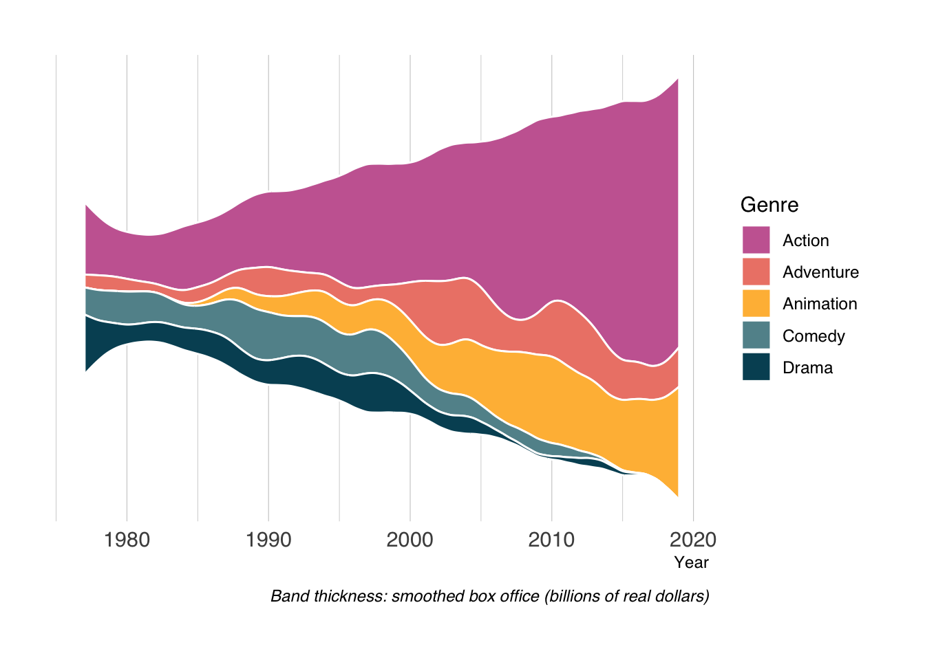
A streamgraph moves the baseline and smooths the bands. It can show broad changes in composition, but the vertical position of a band does not represent its value. Read band thickness, and use a stacked area plot or faceted lines when exact amounts matter. Smoothing may also suggest changes between the observed years.
blockbusters |>
    ggplot(aes(x = year, y = box_office, fill = genre)) +
    labs(
        x = "Year", y = NULL, fill = "Genre",
        caption = "Band thickness: smoothed box office (billions of real dollars)"
    ) +
    ggstream::geom_stream(color = 'white') +
    MetBrewer::scale_fill_met_d("Cross") +
    theme(
        axis.text.y = element_blank(),
        axis.ticks.y = element_blank(),
        panel.grid.major.y = element_blank(),
        panel.grid.minor.y = element_blank()
    )
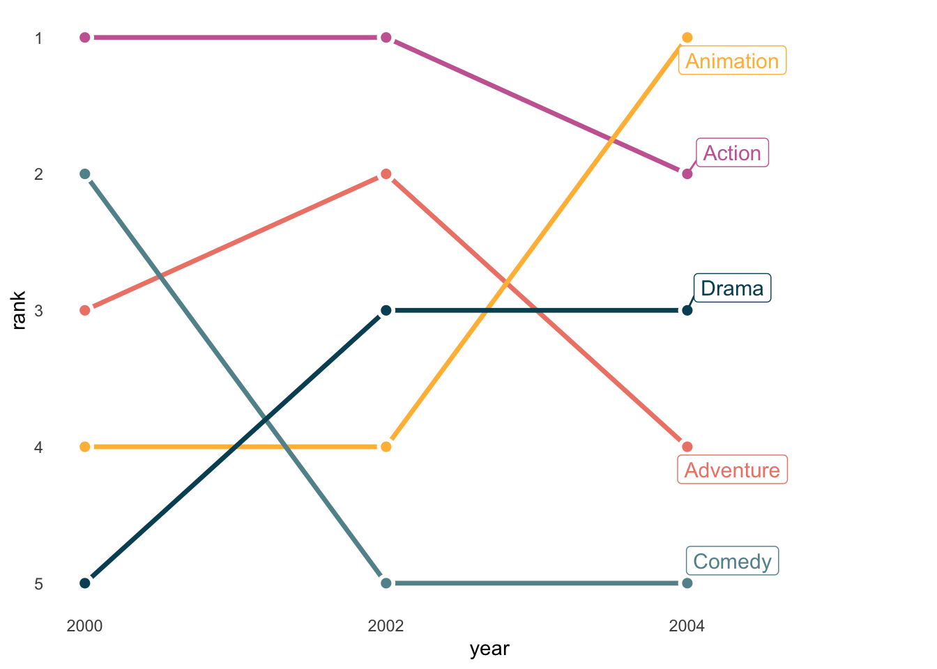
Bump charts show changes in rank for a small number of groups. They discard the size of the differences: ranks 1 and 2 can be almost tied or far apart. We can draw one with ordinary ggplot2 lines and points. The connections below link only the selected years; they do not show observed rankings in the intervening years.
blockbusters |>
filter(year %in% c(2000, 2002, 2004)) |>
group_by(year) |>
mutate(rank = min_rank(desc(box_office))) |>
ungroup() |>
ggplot(aes(x = year, y = rank, color = genre)) +
geom_line(linewidth = 1.2) +
geom_point(color = "white", size = 4) +
geom_point(size = 2) +
ggrepel::geom_label_repel(data = \(d) filter(d, year == 2004), aes(label = genre),
size = 4, nudge_x = 0.3, direction = "y", seed = 234) +
MetBrewer::scale_color_met_d("Cross") +
scale_x_continuous(breaks = c(2000, 2002, 2004), expand = expansion(mult = c(0.05, 0.3))) +
scale_y_reverse(breaks = 1:5) +
theme_minimal() +
theme(legend.position = 'none',
panel.grid = element_blank()
)- 1
-
min_rank(desc(box_office))gives rank 1 to the largest value. Ties share a rank and leave a gap in the next rank; choose and explain a tie rule when ties occur. - 2
- Put rank 1 at the top, the usual convention for bump charts.
A third axis adds perspective and occlusion when the groups are merely categories. Rotate this example and compare how easy it is to judge values against the faceted plots above. The interactive plot needs HTML output; it will not appear in a static PDF.
blockbusters |>
    plotly::plot_ly(x = ~year,
        y = ~genre,
        z = ~box_office,
        type = 'scatter3d',
        mode = 'lines',
        color = ~genre)
13.4 Choosing a Trend Plot
| Question | Useful starting point |
|---|---|
| What changed between observations? | Points connected by straight lines |
| What is the longer-term pattern? | Observations plus a clearly specified moving average or smoother |
| How do group trajectories compare? | Facets with shared axes, or a few labeled lines |
| How do groups contribute to a total? | Stacked areas with a zero baseline |
| How did the ordering change? | A bump chart with an explicit tie rule |