pak::pak(c("tidyverse", "janitor", "scales", "palmerpenguins", "cowplot", "ggdensity", "ggside", "modeldata", "scattermore", "ggpointdensity", "Sleuth3", "ggpmisc", "GGally", "ggpca"))14 Visualizing Association
Class Objectives:
- Read associations within and across groups
- Handle overplotting and show marginal distributions
- Interpret transformed axes and fitted relationships
- Explore several variables with pairwise plots and PCA
Packages for this chapter
If you haven’t installed the following packages, run this code:
Association plots describe how variables vary together. Look for direction, form, strength, outliers, and differences between groups. A visual association alone does not establish causation.
We continue the same workflow: load tidyverse and palmerpenguins to use their functions and data directly, clean names with janitor::clean_names(), and use package::function() for other packages.
library(tidyverse)
library(palmerpenguins)
theme_set(cowplot::theme_cowplot())

penguins_clean <- penguins |>
    janitor::clean_names()

penguins_bills <- penguins_clean |>
    drop_na(bill_length_mm, bill_depth_mm, species)
14.1 Start with a Scatter Plot
For the bill measurements, remove rows missing either plotted variable. This keeps the scatter plots, smoothers, and marginal densities on the same set of observations. State which rows you omit; missing values may themselves have a pattern.
penguins_bills |>
    ggplot(aes(x = bill_length_mm, y = bill_depth_mm)) +
    geom_point(alpha = 0.6) +
    labs(x = "Bill length (mm)", y = "Bill depth (mm)")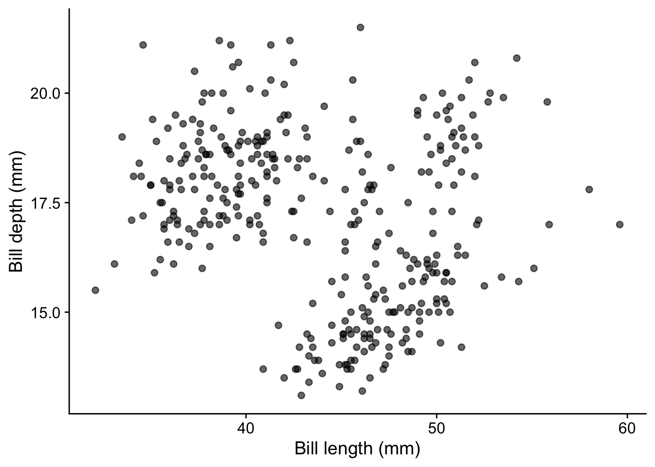
Before interpreting a pooled pattern, check whether it combines distinct groups. Mapping species to color lets us inspect the within-species relationships. The mapping also makes geom_smooth() fit one line per species:
penguins_bills |>
    ggplot(aes(x = bill_length_mm, y = bill_depth_mm, color = species)) +
    geom_point(alpha = 0.6) +
    geom_smooth(method = "lm", formula = y ~ x, se = FALSE) +
    labs(x = "Bill length (mm)", y = "Bill depth (mm)", color = "Species")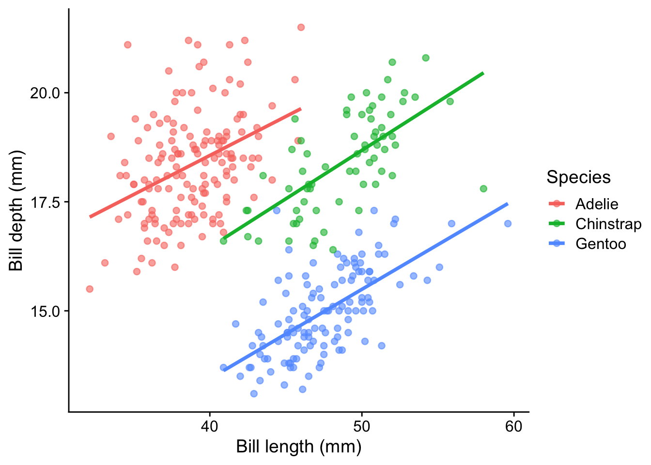
The overall relationship can differ from those within groups. These straight lines are descriptive summaries; inspect the point clouds before choosing a linear model.
14.2 Marginal distributions
Marginal distributions show the distribution of each variable along the axes of a scatter plot. They provide additional context to understand the spread and density of the data.
A simple way to add marginal information is by using geom_rug(), which adds tick marks along the axes:
penguins_bills |>
    ggplot(aes(x = bill_length_mm, y = bill_depth_mm)) +
    geom_point() +
    geom_rug()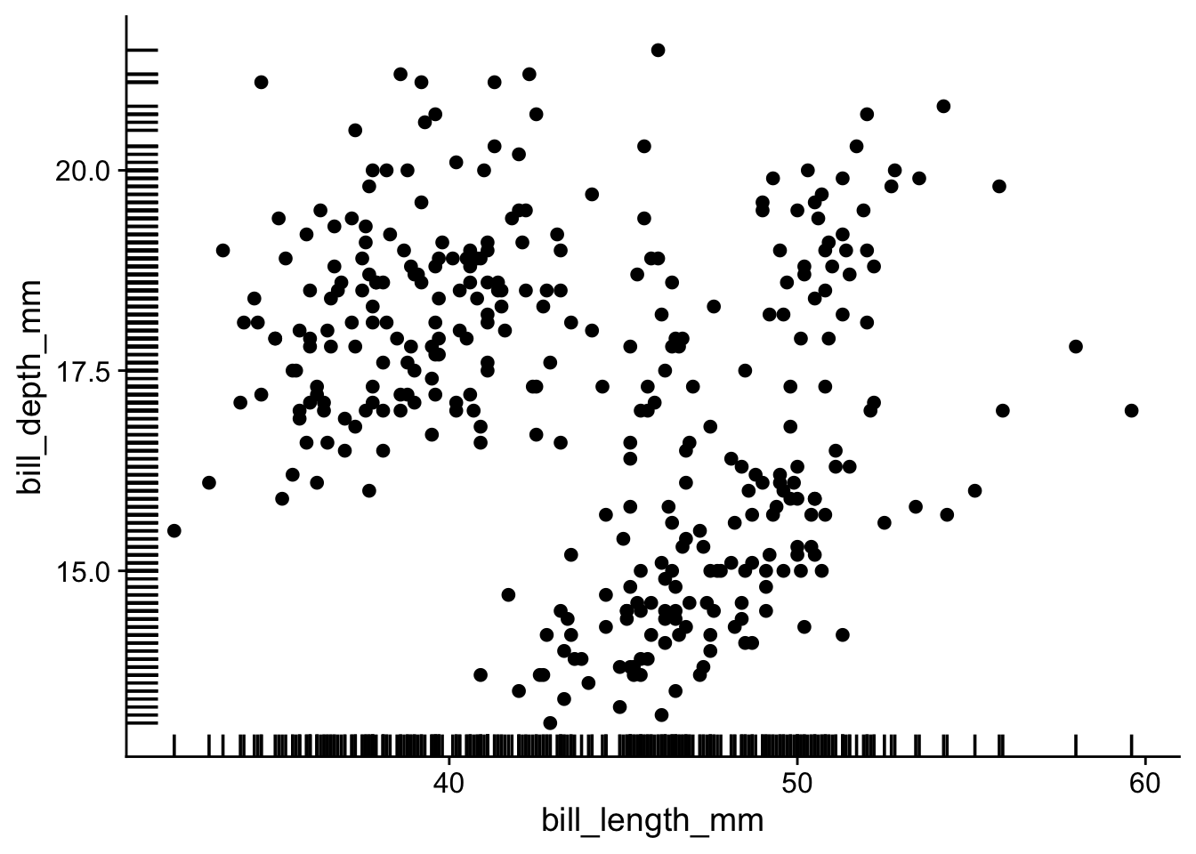
With many points, it becomes difficult to see the marginal distributions. I prefer to use geom_hdr_rug() from ggdensity package:
penguins_bills |>
    ggplot(aes(x = bill_length_mm, y = bill_depth_mm)) +
    geom_point() +
    ggdensity::geom_hdr_rug()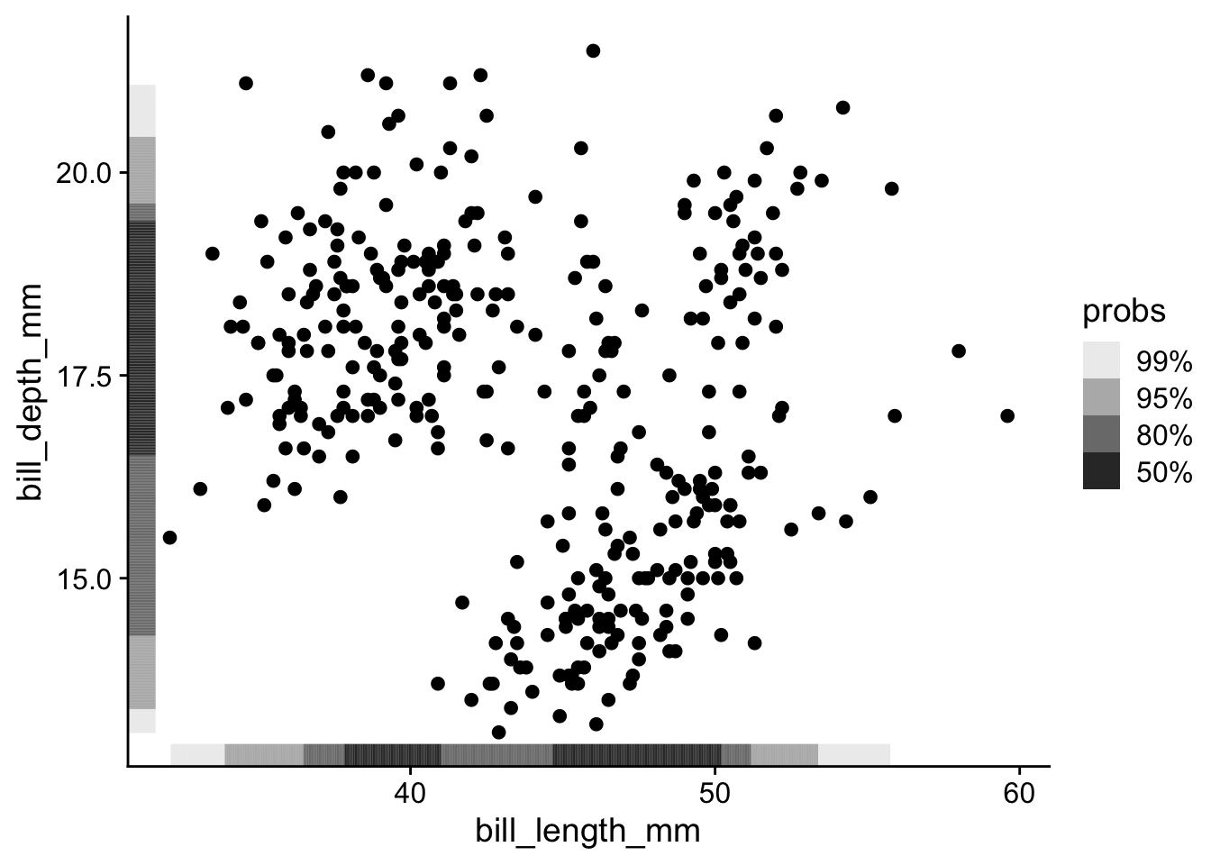
Rug marks overlap when there are many observations or groups.
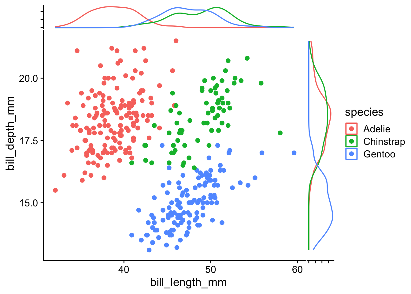
For a clearer view by group, ggside adds density plots along each axis. These densities describe each variable separately; they do not describe the association between the pair. Each group’s density integrates to one, so density height does not directly indicate group size.
penguins_bills |>
ggplot(aes(x = bill_length_mm, y = bill_depth_mm, color = species)) +
geom_point() +
ggside::geom_xsidedensity(aes(y = after_stat(density))) +
ggside::geom_ysidedensity(aes(x = after_stat(density))) +
theme(
ggside.axis.text = element_blank()
)- 1
- Add density plot along the x-axis
- 2
- Add density plot along the y-axis
- 3
- Remove side axis text
14.3 Addressing Overplotting
When there are too many points in a scatter plot, overplotting can obscure patterns and lead to misinterpretation (for a discussion of a real controversy in which plotting choices mattered, see this blog post).
Use modeldata::lending_club to compare displays for a larger dataset. First clean its names, then retain finite, strictly positive values for the two variables we will log-transform. A logarithm cannot represent zero or negative values. We report the number excluded and create new columns so the original measurements remain available.
lending_club_clean <- modeldata::lending_club |>
    janitor::clean_names()

lending_club_positive <- lending_club_clean |>
    filter(
        is.finite(annual_inc), annual_inc > 0,
        is.finite(total_il_high_credit_limit), total_il_high_credit_limit > 0
    )

nrow(lending_club_clean) - nrow(lending_club_positive)
[1] 1096lending_club_log10 <- lending_club_positive |>
mutate(
log10_annual_inc = log10(annual_inc),
log10_credit_limit = log10(total_il_high_credit_limit)
)
lending_club_log10 |>
ggplot(aes(x = log10_annual_inc, y = log10_credit_limit)) +
labs(x = "log10(annual income / USD)", y = "log10(installment credit limit / USD)") +
geom_point()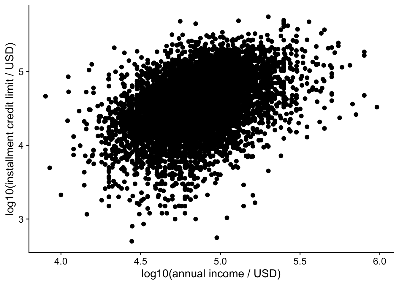
These plots describe only observations with positive values for both measurements. Zero credit limits remain meaningful in the original data and would need a different display if they are part of the question.
Lower alpha makes points more transparent, allowing dense regions to accumulate more visible ink:
lending_club_log10 |>
ggplot(aes(x = log10_annual_inc, y = log10_credit_limit)) +
labs(x = "log10(annual income / USD)", y = "log10(installment credit limit / USD)") +
geom_point(alpha = 0.05)- 1
- Set opacity: 0 is fully transparent and 1 is fully opaque.
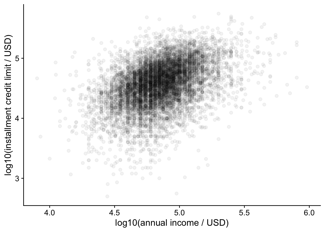
For example, with alpha = 0.05 each point is 5% opaque, so it takes roughly 20 overlapping points before an area looks about 64% opaque (1 - 0.95^20), and around 60 to reach 95%.
A two-dimensional histogram counts observations in rectangular cells. This is useful when the question is how many observations occupy each region, and avoids drawing thousands of overlapping points.
lending_club_log10 |>
    ggplot(aes(x = log10_annual_inc, y = log10_credit_limit)) +
    geom_bin_2d(bins = 35) +
    scale_fill_viridis_c(trans = "sqrt", name = "Count") +
    labs(x = "log10(annual income / USD)", y = "log10(installment credit limit / USD)")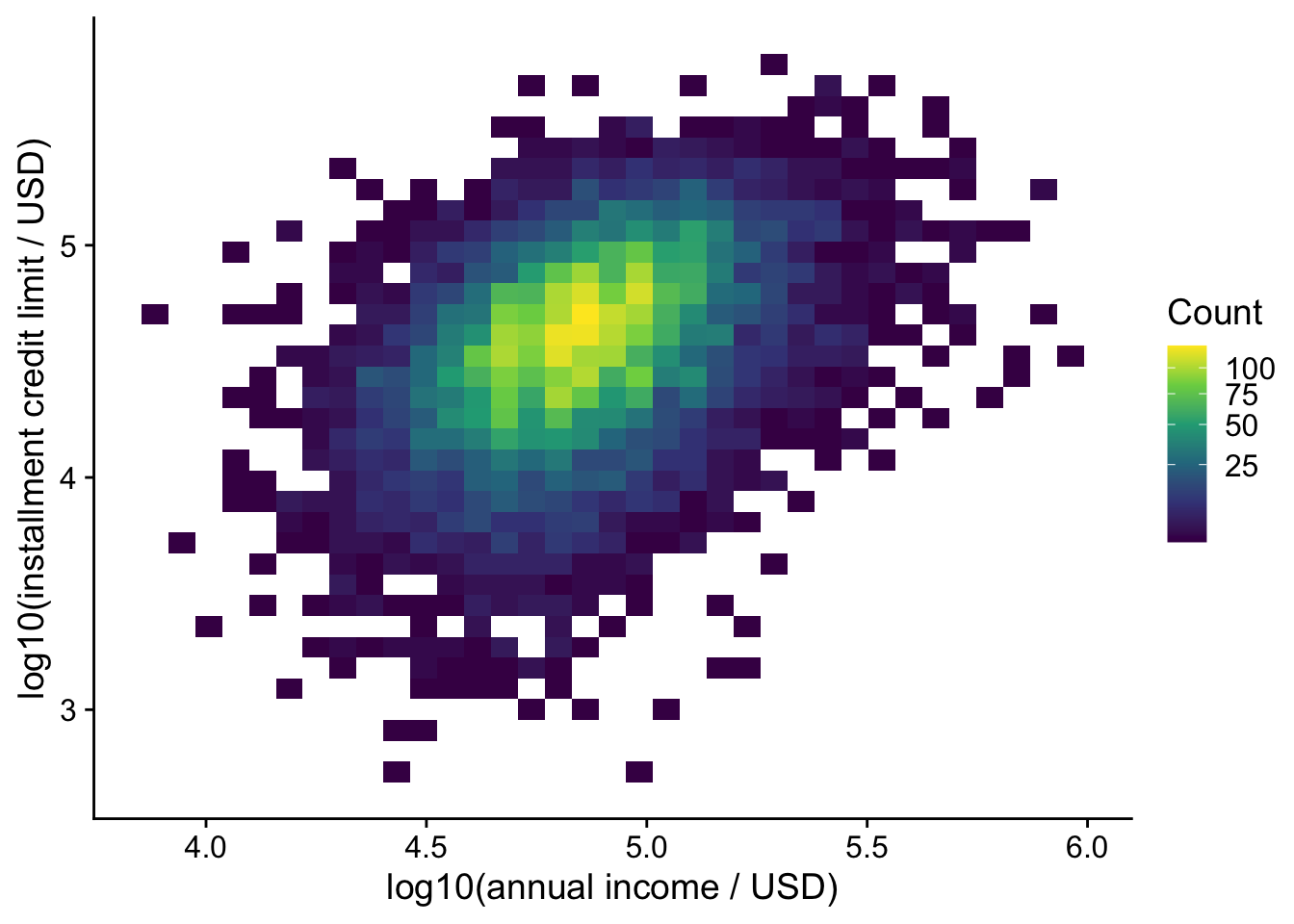
Compare several bin counts, just as you would for a one-dimensional histogram. The square-root color transformation makes smaller counts easier to see; the legend still reports counts. Here the bins are in log-transformed coordinates, so equal widths correspond to equal ratios in the original measurements. See the geom_bin_2d() documentation.
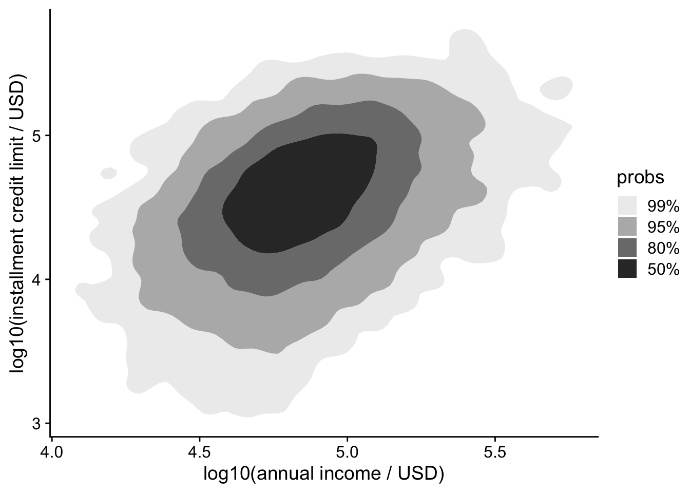
Instead of plotting every individual point, you can visualize the density of points using contour plots. We will use the ggdensity package to help with this.
lending_club_log10 |>
ggplot(aes(x = log10_annual_inc, y = log10_credit_limit)) +
labs(x = "log10(annual income / USD)", y = "log10(installment credit limit / USD)") +
ggdensity::geom_hdr()- 1
- Show estimated highest-density regions: the legend gives the probability mass enclosed by each region. These are regions of the fitted distribution, not confidence intervals for a regression line.
Alternatively, you can overlay density contours on top of a scatter plot:
lending_club_log10 |>
ggplot(aes(x = log10_annual_inc, y = log10_credit_limit)) +
labs(x = "log10(annual income / USD)", y = "log10(installment credit limit / USD)") +
geom_point(shape = '.', color = 'black', alpha = 0.3) +
ggdensity::geom_hdr_lines()- 1
- Draw small, partially transparent points.
- 2
- Draw density contours last so they remain visible.
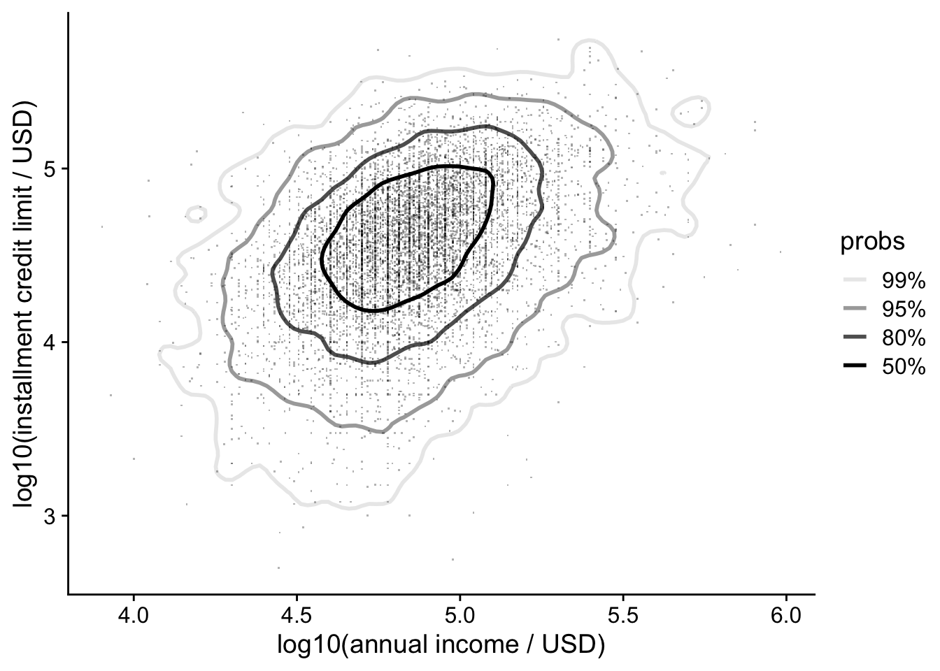
The dot symbol shape = "." draws very small points whose appearance depends on the output device. Check the exported figure at its intended size. Density contours also depend on the smoothing bandwidth; they can hide small clusters or create a misleading impression of separation.
Want it even faster?
For larger datasets, scattermore::geom_scattermore() rasterizes the point layer. It can reduce rendering time and output size, while the surrounding axes and text remain separate plot elements.
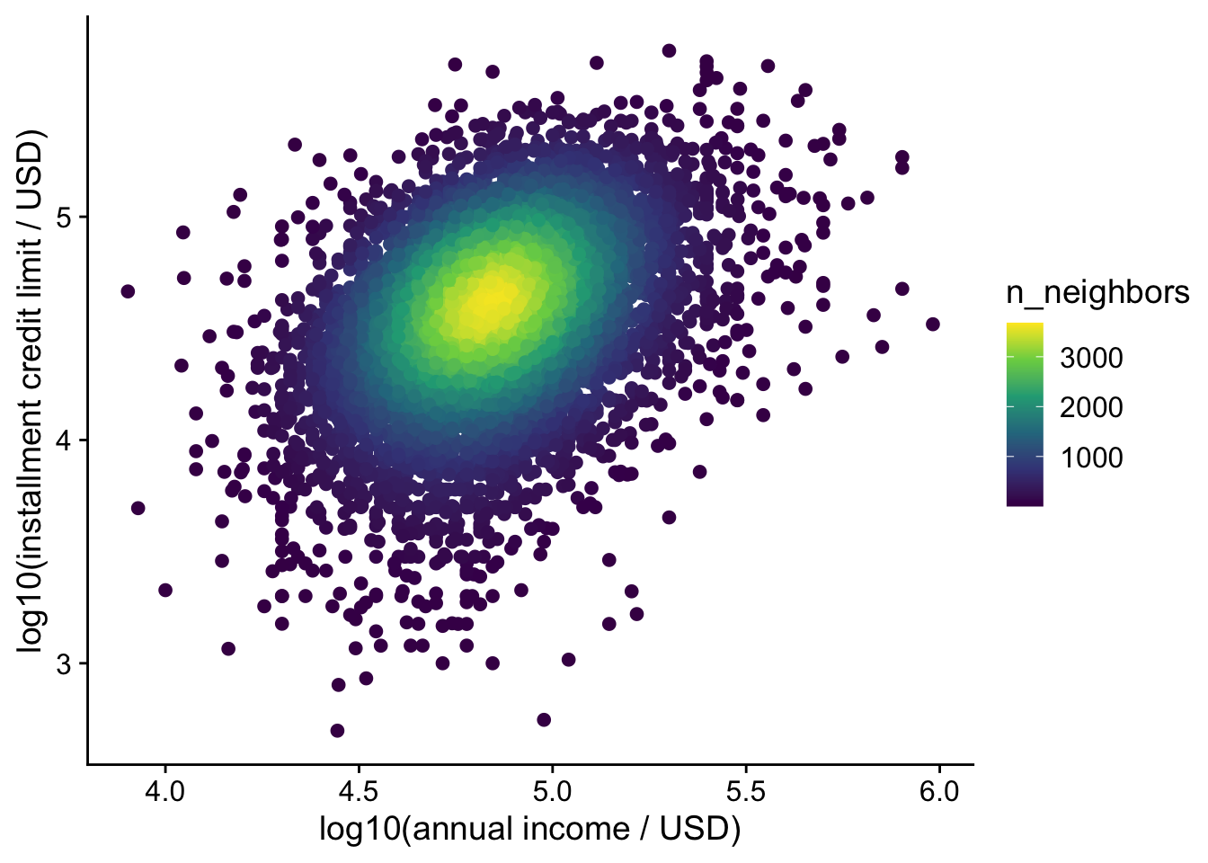
The ggpointdensity package colors points based on the local point density, highlighting areas of high concentration. It combines the best of both worlds: individual points and a density estimate.
lending_club_log10 |>
ggplot(aes(x = log10_annual_inc, y = log10_credit_limit)) +
labs(x = "log10(annual income / USD)", y = "log10(installment credit limit / USD)") +
ggpointdensity::geom_pointdensity() +
scale_color_viridis_c()- 1
- Use viridis color palette (generally preferred over the default)
14.4 Axis Transformation
A log axis is useful when ratios matter or values span orders of magnitude. Equal distances represent equal ratios: going from 1 to 10 occupies the same distance as going from 10 to 100. Unlike the manually transformed columns above, scale_x_log10() and scale_y_log10() keep axis tick labels in the original units. Do not apply them again to columns already containing logarithms.
The Sleuth3::ex0826 dataset contains average body mass (kg) and metabolic rate (kJ/day) for 95 mammal species. Clean its names before plotting: Mass becomes mass and Metab becomes metab.
Kleiber’s law proposes a relationship of the form \(\mathrm{metab} = a\,\mathrm{mass}^{b}\) with \(b \approx 3/4\). Taking logs gives \(\log_{10}(\mathrm{metab}) = \log_{10}(a) + b\log_{10}(\mathrm{mass})\), so the slope on log–log axes estimates the exponent.
metabolism <- Sleuth3::ex0826 |>
janitor::clean_names()
metabolism |>
ggplot(aes(x = mass, y = metab)) +
geom_point() +
scale_x_log10(
breaks = scales::trans_breaks("log10", function(x) 10^x),
labels = scales::trans_format("log10", scales::math_format(10^.x))
) +
scale_y_log10(
breaks = scales::trans_breaks("log10", function(x) 10^x),
labels = scales::trans_format("log10", scales::math_format(10^.x))
) +
annotation_logticks() +
labs(x = "Body mass (kg; log scale)", y = "Metabolic rate (kJ/day; log scale)") +
geom_smooth(method = "lm", formula = y ~ x) +
ggpmisc::stat_poly_eq(
ggpmisc::use_label(c("eq", "R2")), formula = y ~ x,
eq.with.lhs = "log[10](metab)~~`=`~~",
eq.x.rhs = "log[10](mass)"
)- 1
- The ordinary least squares line, fitted on the log-transformed values.
- 2
- Print the fitted equation and R², explicitly labeling the logarithms in the equation. The slope is the estimated exponent.
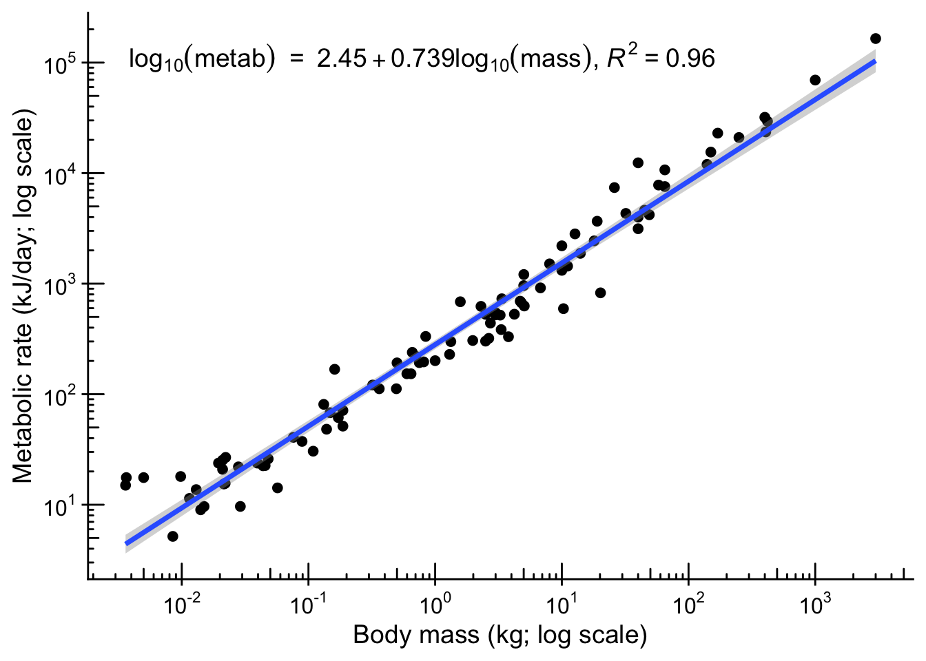
The plot itself does not test anything; to compare the slope with 3/4 we need its confidence interval:
metabolism_fit <- stats::lm(log10(metab) ~ log10(mass), data = metabolism)
stats::confint(metabolism_fit, parm = "log10(mass)")
2.5 % 97.5 %
log10(mass) 0.7097121 0.7677752The 95% confidence interval for the slope (log10(mass)) is about 0.71 to 0.77 and includes 0.75. Under this linear model’s assumptions, the data are compatible with that exponent; they do not prove an exact universal value. A biological analysis should also assess residuals and dependence among related species.
State the transformation and units in the labels. A straight line after transformation describes a relationship on that transformed scale; its interpretation on the original scale must follow the transformation. See this discussion of log transformations.
A strong-looking association or large R² is not evidence of causation. Study design, model assumptions, and plausible confounding variables still matter; related scientific debates are discussed here and here.
14.5 High-Dimensional Data
When dealing with multiple variables, it is often insightful to explore relationships beyond simple 2D plots. We illustrate two common approaches with the penguins dataset.
penguins_small <- penguins_clean |>
    select(species, bill_length_mm, bill_depth_mm, flipper_length_mm, body_mass_g) |>
    drop_na()
14.5.1 Pairwise plots
Pairwise plots (or scatterplot matrices) allow you to visualize the relationships between all pairs of variables in a dataset. They are especially useful for exploratory data analysis. We will use the GGally package to create these plots.
penguins_small |>
    GGally::ggpairs(
        columns = 2:5,
        mapping = aes(color = species, alpha = 0.5),
        upper = list(continuous = GGally::wrap("cor", stars = FALSE))
    )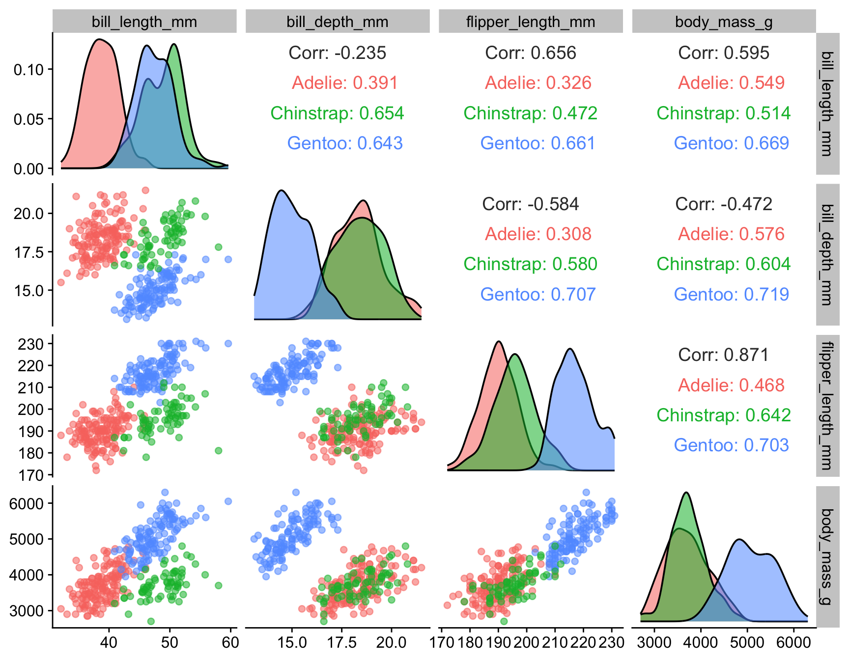
The matrix includes the four numerical measurements; species is used only for color. Compare patterns within species with the pooled pattern, and treat the matrix as exploration rather than a collection of independent significance tests.
14.5.2 Dimension reduction
Principal component analysis (PCA) projects numerical measurements onto axes that capture as much variation as possible. Use the same complete observations as in the scatterplot matrix. Here species supplies labels and colors; it is excluded from the numerical features used to compute the components. The ggpca package draws the result.
penguins_small |>
ggpca::ggpca(
metadata_cols = "species",
mode = "pca",
scale = TRUE,
color_var = "species",
ellipse = TRUE,
ellipse_level = 0.9,
ellipse_type = "norm"
)- 1
- Column to use for grouping/metadata
- 2
- Compute PCA from the numerical measurements; scaling is explicit because their units differ.
- 3
- Color points by species
- 4
- Add ellipses (by default, 90% normal-theory ellipses that describe the spread of each group; they are not boundaries that separate groups)
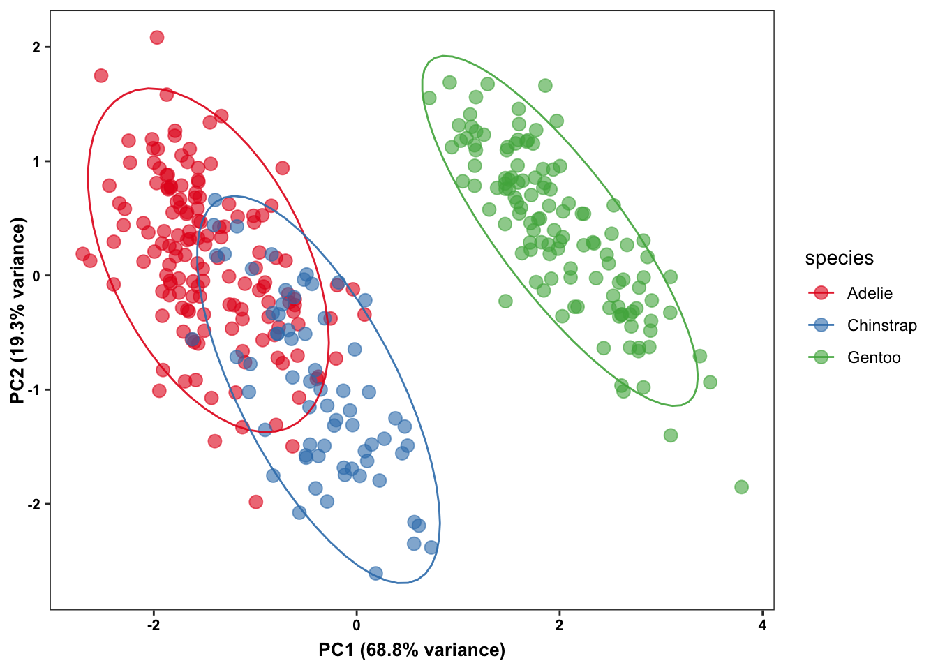
With scale = TRUE, the PCA standardizes each measurement to unit variance. Without scaling, the much larger numerical variance of body mass in grams would dominate the analysis. Inspect the explained variance and loadings to understand what the two-dimensional plot retains:
penguins_pca <- penguins_small |>
    select(-species) |>
    stats::prcomp(center = TRUE, scale. = TRUE)

summary(penguins_pca)$importance
PC1 PC2 PC3 PC4
Standard deviation 1.659444 0.8789293 0.6043475 0.3293816
Proportion of Variance 0.688440 0.1931300 0.0913100 0.0271200
Cumulative Proportion 0.688440 0.8815700 0.9728800 1.0000000penguins_pca$rotation[, 1:2] PC1 PC2
bill_length_mm 0.4552503 -0.597031143
bill_depth_mm -0.4003347 -0.797766572
flipper_length_mm 0.5760133 -0.002282201
body_mass_g 0.5483502 -0.084362920The variance proportions describe how much of the standardized data variation each component captures. The loadings describe each original variable’s contribution to a component; the overall sign of a component is arbitrary.
The package also supports t-SNE and UMAP, but switching methods changes the meaning of the display. Those methods depend on tuning choices and randomness; set a seed and inspect sensitivity when using them. Distances between apparent clusters in their two-dimensional output need not represent distances in the original data. See this discussion of dimension-reduction pitfalls.
14.6 Choosing an Association Plot
| Question | Useful starting point |
|---|---|
| How do two measurements vary together? | Scatter plot, with relevant groups identified |
| What are the separate distributions? | Marginal rugs or densities |
| Where do many observations overlap? | Transparent points, 2D counts, or density contours |
| Is the relationship multiplicative? | Log axes with explicit units and a justified model |
| How do several measurements relate? | Scatterplot matrix, then PCA with variance and loadings |