library(tidyverse)
library(palmerpenguins)21 Tibble-centric Workflow for Simulation
Class Objectives
- Master thw workflow of simulation in data analysis
- Learn how to implement bootstrap resampling
- Learn how to simulate population dynamics
21.1 Organization Simulation
Simulation can cover everything from simple statistical tests to differential equations or even complex individual-based models. We won’t dive into every type here, but it’s important to know how to structure your simulation so that your analysis stays organized and reproducible. In our examples, we’ll stick with the tibble as our main data structure.
21.2 Bootstrap: Your Statistical Superpower
Ever been asked, “How sure are you about that number?” and wished you could give a more precise answer than “Pretty sure”? That’s where simulation—and specifically bootstrap—comes in.
Imagine being able to collect your data again and again—even if you only have one sample. Bootstrap lets you do just that by resampling your original data many times. Here’s how it works in plain English:
- Resample: Randomly pick data points from your original sample (with replacement, so you might pick the same point more than once).
- Calculate: Compute the statistic you’re interested in (like the mean or median) on each resample.
- Repeat: Do this many times.
- Summarize: Look at the distribution of your computed statistics to gauge your uncertainty.
21.2.1 Example: How Heavy Are These Penguins, Really?
Let’s start by checking out the average body mass for each penguin species:
# Let's see what we're working with
penguins |>
    group_by(species) |>
    summarise(
        mean_body_mass = mean(body_mass_g, na.rm = TRUE)
    )
Cool, but how confident are we in these averages? Let’s use bootstrap to find out!
n_bootstraps <- 100
penguins_bootstrapped <- penguins |>
select(species, body_mass_g) |>
group_by(species) |>
nest() |>
expand_grid(
bootstrap_id = 1:n_bootstraps
) |>
mutate(
bootstrap_sample = map(data, \(x) sample_n(x, size = nrow(x), replace = TRUE))
) |>
mutate(
mean_body_mass = map_vec(bootstrap_sample, ~ mean(.x$body_mass_g, na.rm = TRUE))
)- 1
- Let’s do 1,000 bootstrap samples (why not?)
- 2
- Just grab what we need
- 3
- Group by species (we want separate bootstraps for each)
- 4
- Nest the data (create a tibble for each species)
- 5
- Create 1,000 bootstrap samples for EACH species
- 7
- Calculate the mean for each bootstrap sample
Here’s what we did:
- Select: We kept only the columns we need.
- Group & Nest: Each species’ data gets its own little tibble.
- Expand: We create 100 copies of the data for each species.
- Resample: We randomly sample (with replacement) from each species’ data.
- Calculate: For each bootstrap sample, we compute the mean body mass.
Now, let’s summarize our bootstrap results:
penguins_bootstrapped |>
group_by(species) |>
summarise(
mean_estimate = mean(mean_body_mass),
se_estimate = sd(mean_body_mass),
lower_ci = quantile(mean_body_mass, 0.025),
upper_ci = quantile(mean_body_mass, 0.975)
)- 1
- Group by species
- 2
- Calculate the mean estimate
- 3
- Calculate the standard error
- 4
- Calculate the lower confidence intervals
- 5
- Calculate the upper confidence intervals
And let’s visualize the bootstrap distributions:
#penguins_bootstrapped
penguins_bootstrapped  |>
    ggplot(aes(x = mean_body_mass, fill = species, color = species)) +
    geom_density(alpha = 0.5) +
    labs(
        title = "Bootstrap Distributions of Mean Body Mass",
        subtitle = "Each curve shows 1,000 bootstrap samples - look at all that uncertainty!",
        x = "Mean Body Mass (g)",
        y = "Density"
    ) +
theme_minimal() 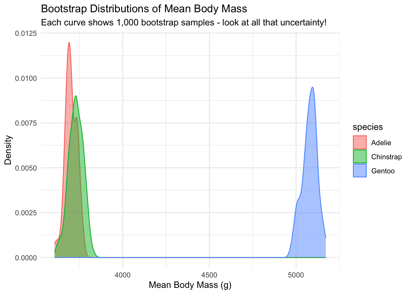
21.2.2 What Just Happened? The Bootstrap Breakdown
Let’s break down what we did with our bootstrap code:
- Data Nesting: We grouped by species and nested the data (like putting each species’ data in its own little box)
- Bootstrap Creation: We used
expand_grid()to make 1,000 copies of each species’ box - Resampling: We used
map()to randomly grab data from each box (with replacement) - Calculating: We found the mean for each bootstrap sample
- Summarizing: We calculated the average mean, standard error, and confidence intervals
Most importantly, this workflow works for other statistics too! The only thing specific here is the third step, and you can replace it with any other complex operations like uncertainty for regression coefficients, etc.
Exercise: Bootstrap the Median!
Now it’s your turn! Try bootstrapping to estimate the median flipper length for each species.
21.3 Chaos Theory: When Tiny Changes Make a Huge Difference!
Ever heard the saying about a butterfly flapping its wings in Brazil causing a tornado in Texas? That’s chaos theory in action! We’ll explore this concept using a classic example: the logistic map.
The logistic map is a simple equation that can generate wildly complex behavior, often used to model population growth with limited resources. Mathematically, it looks like this: \[x(t+1) = r x(t) (1-x(t))\]
where \(x(t)\) is the population at time \(t\), and \(r\) is a parameter that controls the growth rate.
Let’s write a function to simulate the logistic map:
# This function simulates the logistic map equation:
# x(t+1) = r*x(t)*(1-x(t))
# We're using r=4, which produces chaotic behavior
simulate_logistic <- function(init_condition, total_time) {
population <- c(length = total_time)
population[1] <- init_condition
for (t in 2:total_time) {
population[t] <- 4 * population[t-1] * (1 - population[t-1])
}
tibble(time = 1:total_time,
population = population)
}- 1
- Create an empty vector to store our population values
- 2
- Set the initial condition
- 3
- Calculate each new population value based on the previous one
- 4
- Return a tidy tibble with time and population
Now, let’s see chaos in action by simulating 10 starting conditions that are nearly identical and watching how they evolve over different time periods:
# Let's create 10 different starting conditions that are VERY close to each other
population_dynamics <- tibble(
init_condition = runif(n = 10, min = 0.49, max = 0.51)
) |>
expand_grid(
total_time = c(5, 10, 50)
) |>
mutate(
trajectory = map2(init_condition, total_time,
\(init, time) simulate_logistic(init, time))
) |>
unnest(trajectory)- 1
- Create 10 different starting conditions that are VERY close to each other
- 2
- For each starting condition, we’ll simulate for 5, 10, and 50 time steps
- 3
- Run our simulation for each combination of starting condition and time
- 4
- Unnest to get all our simulation results in one tidy tibble
Let’s plot the results. Each line represents a different starting condition, and you can see how their paths diverge as time goes on:
population_dynamics |>
    ggplot(aes(x = time, y = population, group = init_condition, color = factor(init_condition))) +
    geom_line() +
    facet_wrap(~total_time, scales = "free_x") +
    labs(
        title = "Chaos in Action: The Butterfly Effect",
        subtitle = "Tiny differences in starting values lead to completely different outcomes over time",
        x = "Time",
        y = "Population",
        color = "Starting Value"
    ) +
    theme_minimal() +
    theme(legend.position = "none")  # The legend gets too crowded with 10 values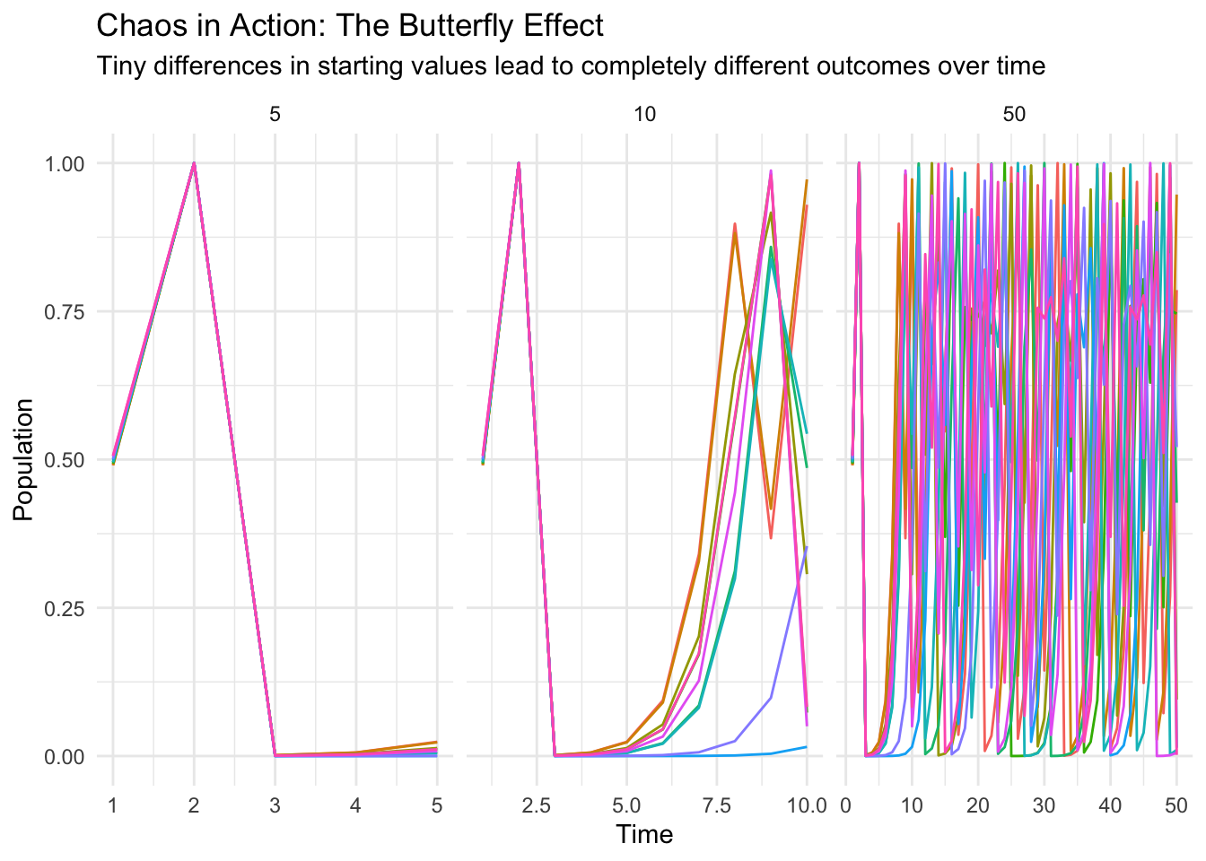
Look at that! In the first 5 time steps, all trajectories follow almost the same path. By 10 time steps, they’re starting to diverge. And by 50 time steps? Complete chaos! The trajectories are totally different, even though the starting conditions were nearly identical.
This is the essence of chaos theory - tiny differences in initial conditions can lead to wildly different outcomes over time. This has huge implications for:
- Weather forecasting (why it’s so hard to predict more than a few days ahead)
- Population biology (why some populations can seem stable, then suddenly crash)
- And many other complex systems!
Exercise: How growth rates modulate dyanmics
Let’s explore how changing the growth rate \(r\) in the logistic map changes the behavior of the system. We’ll simulate the logistic map for different growth rates (2, 3, and 4) and see how the population dynamics evolve over time.
21.4 Summary: Your Simulation Workflow Cheat Sheet
Here’s a quick recap of our simulation workflow:
- Set Up: Create a parameter tibble to define your simulation settings.
- Function: Write a function that performs a single simulation run.
- Functional Programming: Use
map()(orrowwise() + mutate()) to run your simulation across all parameter combinations. - Analyze: Summarize and visualize the results to understand what happened.
Using this structured approach not only saves time and reduces errors but also makes your analysis easier to share and explain.