8 Five verbs for tidying data

Class Objectives: Mastering common tidyr verbs

Reshape data
- pivot_longer(): Transform wide data into a longer, “tall” format.
- pivot_wider(): Transform long data into a wider format.
Split cells
- separate(): Split one column into multiple columns.
Dealing with missing values
- drop_na(): Drop rows with missing values.
- replace_na(): Replace missing values with a specified value.

It’s often said that data cleaning and preparation consume the lion’s share of an analyst’s time—some claim as much as 80%. When real-world data arrives on your desk, chances are it isn’t in a convenient format. Columns may be mislabeled or scattered, variable names might be confusing, and rows may contain missing information. Over the years, analysts have discovered that a consistent “tidy” format for data is invaluable: it lets you focus on extracting insights rather than wrangling columns and rows into submission.

Tidy datasets are all alike, but every messy dataset is messy in its own way. — Hadley Wickham

In practical terms—and echoing our earlier discussion—a tidy dataset has these defining traits:

Every row represents one observation.
Every column represents one variable.
Every cell contains a single value.

The tidyr package (part of the tidyverse) is designed to help transform messy data into this tidy structure. In this chapter, we’ll explore some of the most commonly used tidyr functions, using example datasets that demonstrate where each function shines. We’ll pause our use of the penguins dataset momentarily, because it’s already tidy; instead, we’ll rely on some datasets from dcldata to illustrate typical data-wrangling challenges.

library(tidyverse)
library(tidylog)

# if you haven't installed dcldata, you can do so by running:
# pak::pkg_install("dcl-docs/dcldata")
library(dcldata)

Evolution of Tidying Data in R

Hadley Wickham originally developed the reshape2 package in the 2000s to handle this task. Later, in the tidyr package, he introduced gather() and spread() as an improved approach. These were eventually replaced by pivot_longer() and pivot_wider(), which offer greater clarity and consistency. While the older functions still work, it is recommended to use the newer ones.

8.1 `pivot_longer()`

Let’s begin with the example_eagle_nests dataset from U.S. Fish and Wildlife Service:

example_eagle_nests

Notice that 2017 and 2019 are stored as column names, but they’re really values (i.e., years). This is a classic “wide” format. We can use pivot_longer() to convert it into a tidy format:

eagle_nests_longer <- example_eagle_nests |>
    pivot_longer(
        cols = c(`2007`, `2009`),
        names_to = "year",
        values_to = "nests"
    )
eagle_nests_longer

1: pivot_longer() transforms wide data into a longer, “tall” format.
2: cols specifies the columns to pivot.
3: names_to creates a new column holding the former column names.
4: values_to creates a new column holding the values previously spread across multiple columns.

Why are “year” and “nests” in quotes? Because they are new column names that we are creating. As a general rule, when pivoting, we should always use quotes when creating new columns.

Specifying the columns can sometimes feel like using select(). For instance, you can list the columns to include, or exclude the columns you want to keep untouched. The code below achieves the same result by excluding everything but region:

example_eagle_nests |>
    pivot_longer(
        cols = -c(region), 
        names_to = "year", 
        values_to = "nests" 
    )

Exercise

Try your hand on the billboard dataset (in the tidyverse). This dataset has columns labeled by week (wk1 through wk76), but we want a tidy format that moves those week columns into a single “week” variable and the rankings into another “rank” variable. Use pivot_longer() to make it happen.

Exercise
Solution

8.2 `pivot_wider()`

The pivot_wider() function reverses what pivot_longer() does, turning long datasets into wide formats. Suppose you want to revert our eagle_nests_longer data back to its original shape:

eagle_nests_longer |>
    pivot_wider(
        names_from = "year",
        values_from = "nests"
    )

1: pivot_wider() transforms long data into a wider format.
2: names_from identifies which column contains the new column names.
3: values_from identifies the column whose values will fill the new cells.

Let’s see a more practical example with our penguins dataset. Perhaps we want to compare bill length between male and female penguins for each species. We can create a summary of the mean bill length by species and sex, then convert that summary into a wide layout:

We firstly use our hard-earned data transformation skills to calculate the mean bill length by the groups

library(palmerpenguins)

penguins |>
   group_by(species, sex) |>
   summarise(mean_bill_length = mean(bill_length_mm))

Because comparing values side by side can be clearer, let’s pivot the data wider:

penguins |>
   group_by(species, sex) |>
   summarise(mean_bill_length = mean(bill_length_mm)) |>
   ungroup() |>
   pivot_wider(
      names_from = "sex",
      values_from = "mean_bill_length"
   )

We can go one step further and visualize how male and female bill lengths compare:

penguins |>
   group_by(species, sex) |>
   summarise(mean_bill_length = mean(bill_length_mm)) |>
   ungroup() |>
   pivot_wider(
      names_from = "sex",
      values_from = "mean_bill_length"
   ) |>
   ggplot(aes(male, female)) +
   geom_point(size = 4) +
   ggrepel::geom_text_repel(aes(label = species), box.padding = 1) +
   geom_abline(intercept = 0, slope = 1) +
   jtools::theme_nice()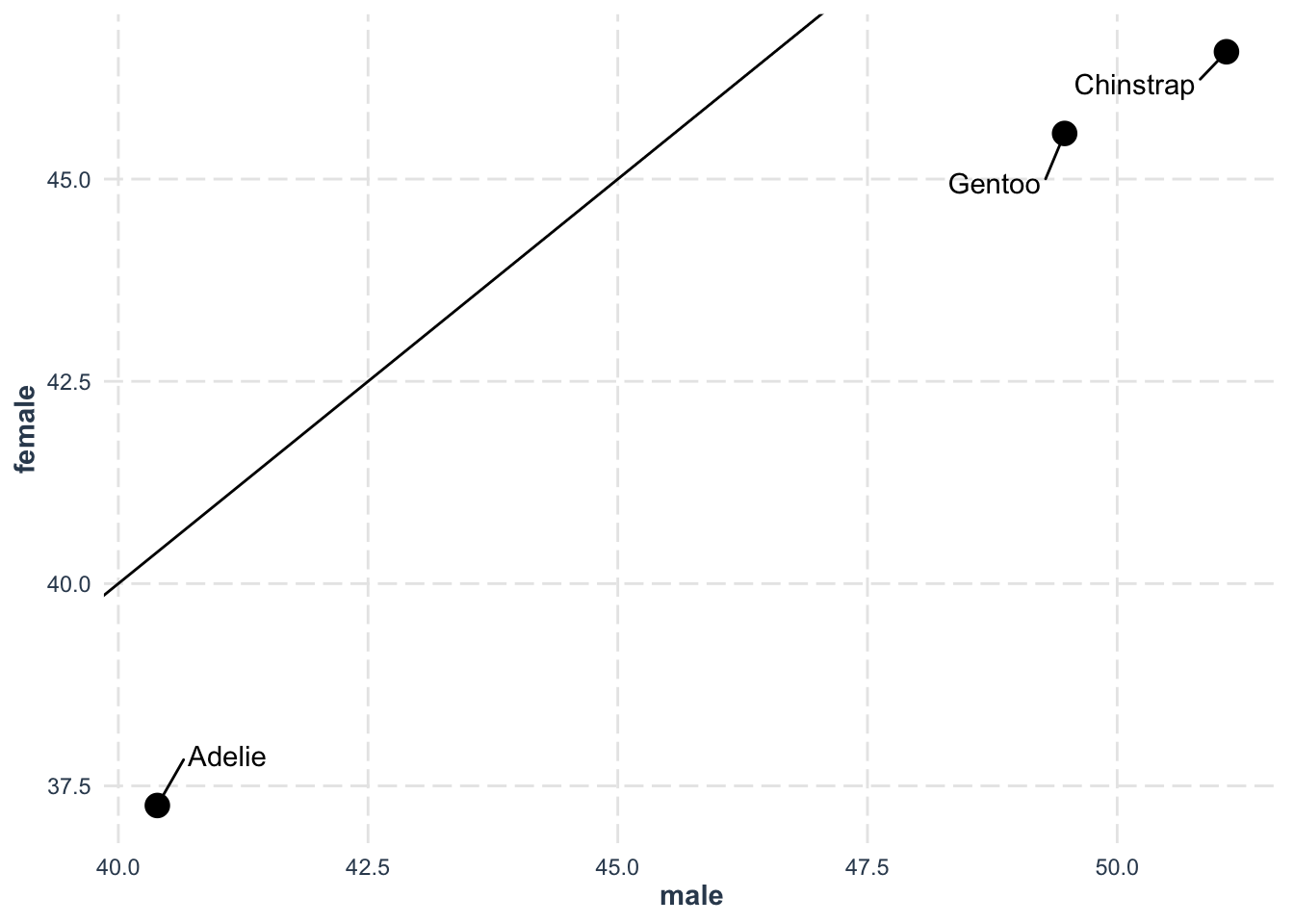

Exercise

The dataset us_rent_income (from the tidyverse) contains 2017 American Community Survey data, where variable indicates whether it’s yearly income or monthly rent, and estimate gives the numeric value. Use pivot_wider() to reshape, then calculate the ratio of annual rent to income, and finally sort the results by that ratio.

Exercise
Solution

8.3 `separate()`

The separate() function allows you to split one column into multiple columns. Consider the example_gymnastics_2 dataset from dcldata, which tracks women’s Olympic gymnastic scores for 2012 and 2016:

example_gymnastics_2

The column names aren’t tidy. First, let’s pivot everything into a long format:

example_gymnastics_2 |>
    pivot_longer(
        cols = -c(`country`), 
        names_to = "eventandyear", 
        values_to = "score"
    )

We see that the new event_year column contains both an event name and a year (like vault_2012). We can split this into two columns—event and year—using separate():

example_gymnastics_2 |>
    pivot_longer(
        cols = -c(`country`), 
        names_to = "eventandyear", 
        values_to = "score"
    ) |>
    separate(
        col = "eventandyear", 
        into = c("event", "year"), 
        sep = "_"
    )

unite()

While separate() splits columns, unite() does the opposite: it combines multiple columns into one.

For a simple example, imagine that we’ve separated out the month, day, and year of a date into three columns (month, day, year), but now we want a single date column again. Let’s illustrate with a small toy dataset:

toy_dates <- tibble(
  month = c(1, 2, 3),
  day   = c(15, 20, 25),
  year  = c(2020, 2020, 2020)
)

We can re-combine these columns into one:

toy_dates |>
  unite(
    col = "full_date",
    month, day, year,
    sep = "-"
  )

1: unite() creates a new column (col = “full_date”) from the listed columns (month, day, year).
2: The new column is named “full_date”.
3: The columns to combine are month, day, and year.
4: sep = “-” indicates how to join the columns (here, with a dash).

Exercise

Now let’s tidy the who2 dataset (from the tidyverse). Columns like sp_m_014 combine multiple pieces of information—diagnosis method (sp), gender (m), and age group (014). Your task:

Convert the data into a long format using pivot_longer().
Split the combined column into three separate columns (diagnosis, gender, age) using separate().

Exercise
Solution

8.4 `drop_na()` and `replace_na()`

When dealing with real-world data, missing values (often represented by NA in R) are unavoidable. It is a very broad topic and usually question-specific. However, we show two functions that help you manage missing data (a really bad story here). The main point is that you should ALWAYS be explict about how you handle missing data.

8.4.1 `drop_na()`

The function drop_na() removes rows that contain any missing values in the specified columns. This can be handy when a row is so incomplete that it’s unusable for analysis.

For example, let’s look at a look from the penguins dataset (pretend we didn’t want to keep partial observations):

penguins

We can drop any row with missing data simply by doing:

penguins |>
  drop_na()

1: drop_na() removes rows with missing values.

drop_na: removed 11 rows (3%), 333 rows remaining

If you only care about missing values in particular columns (say, bill_length_mm), you can specify them as arguments:

penguins |>
  drop_na(bill_length_mm)

1: drop_na() removes rows with missing values in the bill_length_mm column.

drop_na: removed 2 rows (1%), 342 rows remaining

8.4.2 `replace_na()`

Sometimes you don’t want to drop missing values—you might prefer to fill them with a default value or placeholder. The replace_na() function allows you to do exactly that.

For instance, if we believe that the missing sex is most likely to be male, we can replace the missing values with that assumption:

penguins |>
  replace_na(
   list(sex = 'male')
  )

1: Replaces missing values in the sex column as specified.

replace_na: changed 11 values (3%) of 'sex' (11 fewer NAs)

8.5 Tidy a real dataset

Let’s explore the famous Datasaurus dataset, which perfectly illustrates why visualizing your data is crucial (more info). This dataset contains multiple distributions that have identical summary statistics but look completely different when plotted.

library(tidyverse)
# pak::pkg_install("datasauRus")
library(datasauRus)

datasaurus_dozen_wide

1: datasaurus_dozen_wide is the wide format of the Datasaurus dataset.

Let’s tidy this dataset in three steps:

First, we’ll transform it from wide to long format:

datasaurus_dozen_long <- datasaurus_dozen_wide |>
  mutate(row = row_number()) |>
  pivot_longer(
    cols = -"row",
    names_to = "variable",
    values_to = "value"
  )

1: mutate(row = row_number()) adds a row identifier.
2: pivot_longer() pivots the data from wide to long format.
3: names_to creates a new column holding the former column names.
4: values_to creates a new column holding the values previously spread across multiple columns.

mutate: new variable 'row' (integer) with 142 unique values and 0% NA
pivot_longer: reorganized (away_x, away_y, bullseye_x, bullseye_y, circle_x, …) into (variable, value) [was 142x27, now 3692x3]

datasaurus <- datasaurus_dozen_long |>
  separate(
    variable, 
    into = c("dataset", "coord"),
    sep = "_(?=[^_]*$)"
  ) |>
  pivot_wider(
    names_from = "coord", 
    values_from = "value"
  )

1: Split at last underscore
2: pivots the data from long to wide format.

pivot_wider: reorganized (coord, value) into (x, y) [was 3692x4, now 1846x4]

datasaurus

Now we can demonstrate why this dataset is famous. First, let’s check the summary statistics:

# Calculate summary statistics for each dataset
datasaurus |>
  group_by(dataset) |>
  summarise(
    mean_x = mean(x),
    mean_y = mean(y),
    sd_x = sd(x),
    sd_y = sd(y),
    cor = cor(x, y)
  )

group_by: one grouping variable (dataset)
summarise: now 13 rows and 6 columns, ungrouped

Despite having nearly identical summary statistics, when we visualize the data, we see that each dataset forms a completely different shape:

# Create faceted scatter plots
datasaurus |>
  ggplot(aes(x, y, color = dataset)) +
  geom_point() +
  facet_wrap(vars(dataset)) +
  jtools::theme_nice() +
  theme(legend.position = "none") +
  labs(title = "Same summary statistics, very different distributions")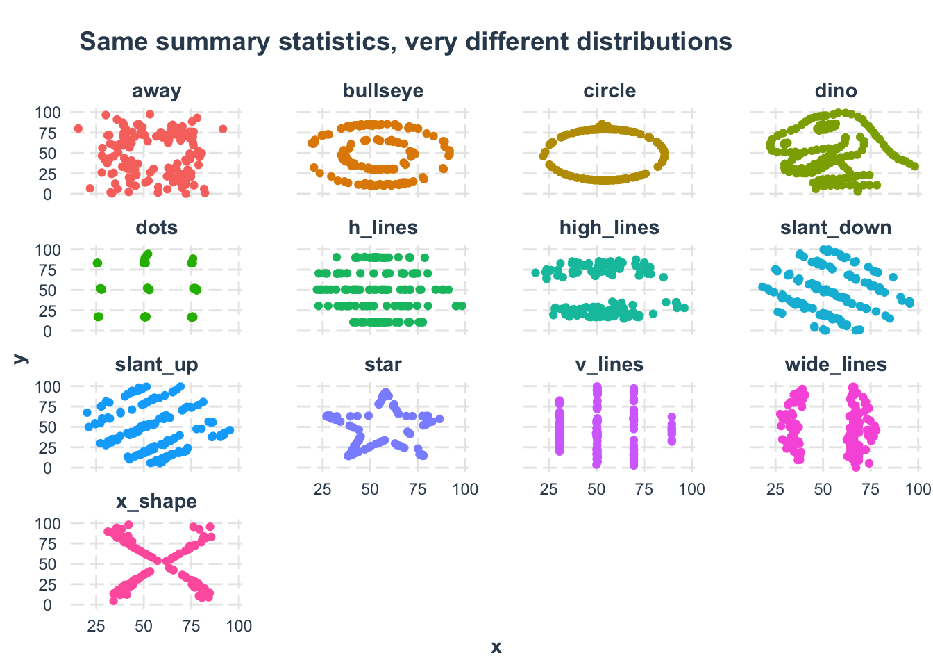

This example demonstrates why it’s essential to both analyze AND visualize your data!

8.1 pivot_longer()

Exercise

8.2 pivot_wider()

Exercise

8.3 separate()

Exercise

8.4 drop_na() and replace_na()

8.4.1 drop_na()

8.4.2 replace_na()

8.5 Tidy a real dataset

8.1 `pivot_longer()`

8.2 `pivot_wider()`

8.3 `separate()`

8.4 `drop_na()` and `replace_na()`

8.4.1 `drop_na()`

8.4.2 `replace_na()`