library(tidyverse)
library(palmerpenguins)
ggplot(penguins, aes(x = bill_length_mm, y = bill_depth_mm, color = species)) +
geom_point(alpha = 0.7) +
theme_minimal() +
labs(x = "Bill Length (mm)", y = "Bill Depth (mm)")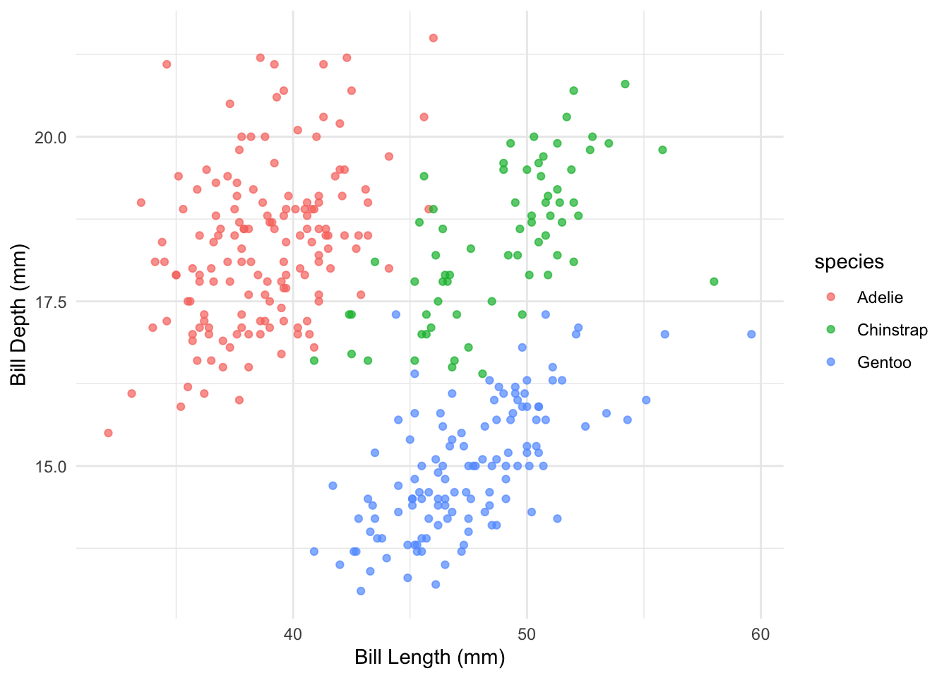
Academic publishing requires precision, consistency, and proper attribution. Quarto excels in these areas by providing:
For academic documents, your YAML header often needs more details:
---
title: "Analysis of Penguin Morphology in the Antarctic Region"
author:
  - name: "Your Name"
    affiliation: "Your University"
    email: "your.email@university.edu"
    orcid: "0000-1234-5678-9101"
  - name: "Co-Author Name"
    affiliation: "Their University"
format: typst
bibliography: references.bib
csl: apa.csl
abstract: |
  This is the abstract of your paper. It should be concise and explain the main
  findings of your work in about 150-250 words.
keywords: [keyword1, keyword2, keyword3]
---
This header provides complete metadata for academic publishing, including proper author information, citation style, and document formatting.
Quarto gives you two engines for producing PDF documents. Both accept the same Markdown source—the difference is under the hood.
LaTeX has been the gold standard for academic typesetting for decades. To use it in Quarto:
format:
  pdf:
    documentclass: article
    classoption: [11pt]
    toc: true
    number-sections: true
    cite-method: biblatex
Importantly, this route requires you to install a LaTeX distribution. The easiest way is to run the following command once in R:
tinytex::install_tinytex()LaTeX has an enormous ecosystem of packages and journal templates, but it can be slow to compile and its error messages are notoriously cryptic.
Typst is a modern typesetting system built from the ground up as a faster, simpler alternative to LaTeX. The great news: Typst is already bundled with Quarto—no extra installation required!
format:
  typst:
    toc: true
    number-sections: true
    columns: 1
Typst compiles in milliseconds where LaTeX takes seconds, and its error messages actually make sense. For course assignments and reports, Typst is the recommended choice.
pdf): Use when a journal requires a specific LaTeX template (e.g., elsarticle, agu-jgr) or you need a niche LaTeX package.One of Quarto’s superpowers is rendering to multiple formats from a single source:
format:
  html: default
  typst:
    toc: true
  docx: default
Run quarto render manuscript.qmd once and you get HTML (for sharing online), PDF (for printing), and Word (for collaborators who need track changes)—all from the same .qmd file.
The first step is to link your bibliography file in the YAML header:
bibliography: references.bib
csl: journal-of-ecology.cslbibliography: Points to your BibTeX or CSL JSON filecsl: (Optional) Specifies the Citation Style Language fileYou can download thousands of CSL style files from zotero.org/styles—just search for your target journal.
Your BibTeX file contains all your references in a structured format. Here’s a sample:
@article{smith2023,
  author = {Smith, John and Johnson, Sarah},
  title = {Analysis of Antarctic Penguin Species Distribution},
  journal = {Journal of Antarctic Biology},
  volume = {45},
  number = {2},
  pages = {112-128},
  year = {2023},
  doi = {10.1234/jab.2023.45.2.112}
}

@book{wilson2020,
  author = {Wilson, Maria},
  title = {Ecological Methodologies in Polar Regions},
  publisher = {Cambridge Academic Press},
  year = {2020},
  isbn = {978-3-16-148410-0}
}.bib FileYou rarely need to type BibTeX entries by hand. Here are the most common workflows:
| Method | How |
|---|---|
| Zotero | Right-click a collection → Export Collection → BibTeX format |
| Google Scholar | Click the " (Cite) button under any paper → BibTeX link |
| DOI lookup | Paste a DOI into doi2bib.org → copy the entry |
| RStudio | Use the Insert Citation (@) dialog—connects directly to Zotero or DOI |
For the smoothest experience, install the Better BibTeX plugin for Zotero. It auto-exports your library to a .bib file that stays in sync whenever you add or edit references.
Once your bibliography is set up, citing sources is straightforward:
According to @smith2023, penguin populations have declined in recent years.

Multiple studies [@smith2023; @wilson2020] have documented this trend.

As Wilson noted [-@wilson2020], methodology is critical in polar research.
These render as:
“According to Smith and Johnson (2023), penguin populations have declined in recent years.”
“Multiple studies (Smith and Johnson, 2023; Wilson, 2020) have documented this trend.”
“As Wilson noted (2020), methodology is critical in polar research.”
Academic papers often require complex mathematical notation. Quarto uses LaTeX syntax for equations, and this works identically in HTML, Typst, and LaTeX output.
For inline equations, use single dollar signs:
The probability is given by $P(X > x) = \int_x^{\infty} f(t) \, dt$For standalone equations, use double dollar signs:
$$
\frac{\partial f}{\partial x} = \lim_{h \to 0} \frac{f(x + h) - f(x)}{h}
$$To create equations you can reference later, use Quarto’s native label syntax:
$$
N(t) = N_0 \, e^{rt}
$$ {#eq-exponential}

See @eq-exponential for the exponential growth model.
Quarto automatically numbers the equation and creates a clickable cross-reference link. This is much simpler than the old LaTeX \tag and \label approach.
For multi-line derivations, use the align environment:
$$
\begin{align}
\frac{dN}{dt} &= rN\left(1 - \frac{N}{K}\right) \\
              &= rN - \frac{rN^2}{K}
\end{align}
$$
Use \\ for line breaks and & to set alignment points (typically before the = sign).
Cross-references help readers navigate your document. Quarto makes this simple with labels and references:
library(tidyverse)
library(palmerpenguins)

ggplot(penguins, aes(x = bill_length_mm, y = bill_depth_mm, color = species)) +
    geom_point(alpha = 0.7) +
    theme_minimal() +
labs(x = "Bill Length (mm)", y = "Bill Depth (mm)")You can then reference this figure: “As shown in Figure 18.1, the bill dimensions clearly differentiate species.”
penguins |>
    group_by(species) |>
    summarise(
        n = n(),
        `Bill Length (mm)` = round(mean(bill_length_mm, na.rm = TRUE), 1),
        `Bill Depth (mm)` = round(mean(bill_depth_mm, na.rm = TRUE), 1)
    ) |>
knitr::kable()| species | n | Bill Length (mm) | Bill Depth (mm) |
|---|---|---|---|
| Adelie | 152 | 38.8 | 18.3 |
| Chinstrap | 68 | 48.8 | 18.4 |
| Gentoo | 124 | 47.5 | 15.0 |
Reference the table in text: “Summary statistics are shown in Table 18.1.”
You can reference sections using their headers:
## Data Collection Methodology {#sec-methodology}

... content ...

As described in @sec-methodology, our approach controls for seasonal variation.
For numbered equations you can reference later:
$$
N(t) = N_0 \, e^{rt}
$$ {#eq-growth}

As shown in @eq-growth, populations grow exponentially when resources are unlimited.| Prefix | What it references | Example |
|---|---|---|
fig- |
Figures | @fig-penguins |
tbl- |
Tables | @tbl-penguin-summary |
sec- |
Sections | @sec-methodology |
eq- |
Equations | @eq-growth |