pak::pak("gt")17 Basics of Quarto
Class Objectives
- The Quarto Setup: Learn about the key parts of a Quarto document.
- Mixing Text, Code, Visuals & Equations: See how you can combine explanations, code, and mathematical formulas in one neat file.
- Making Reproducible Reports: Render your analysis into polished HTML, PDF, or Word documents.
Packages for this chapter
If you haven’t installed the following packages, run this code:
17.1 What’s Quarto All About?
Imagine a tool that lets you write your story and run your code at the same time. That’s Quarto for you! It works with R, Python, Julia, and more, and lets you output to HTML, PDF, Word, presentations, and even websites.
Why should you care?
Because Quarto keeps your analysis, visualizations, and text all in one place. This means anyone can re-run your report and see exactly the same results—making your work truly reproducible and shareable.
17.1.1 A Brief History
The idea of mixing prose and code in one document goes back surprisingly far. Donald Knuth introduced literate programming in the 1980s, arguing that programs should be written for humans to read, not just for machines to execute. In the R world, this philosophy took off with Sweave (2002), which let you embed R code inside LaTeX documents. Then came knitr (2012) by Yihui Xie, which made literate programming much more flexible and user-friendly.
The real game-changer was R Markdown (2014), built on top of knitr and Pandoc. R Markdown made it dead simple to write a document in Markdown, sprinkle in some R code, and render it to HTML, PDF, or Word. It became the standard tool for reproducible research in the R community.
Quarto (2022) is the next evolution, developed by Posit (formerly RStudio). Think of it as R Markdown’s successor—but with a crucial difference: Quarto is language-agnostic. While R Markdown was tightly coupled to R and the knitr engine, Quarto is a standalone tool that works equally well with R, Python, Julia, and Observable JavaScript. Under the hood, Quarto still uses knitr for R code and Jupyter for Python, but the user-facing experience is unified.
17.1.2 Quarto vs. R Markdown
If you’ve used R Markdown before, you’ll feel right at home with Quarto. Here’s the key difference:
| R Markdown | Quarto | |
|---|---|---|
| File extension | .Rmd |
.qmd |
| Languages | Primarily R | R, Python, Julia, Observable |
| Engine |
knitr only |
knitr, Jupyter, or Observable |
| Requires R? | Yes | No (standalone CLI tool) |
| Maintained by | Posit | Posit |
Should I Switch from R Markdown?
If you’re already comfortable with R Markdown, don’t panic—your .Rmd files still work perfectly. But for new projects, Quarto is the way forward. It has better cross-referencing, more output formats, and an active development community. Plus, everything you know about R Markdown (chunk options, YAML headers, Markdown syntax) transfers directly to Quarto.
17.1.3 Installing Quarto
Quarto is a standalone command-line tool—it’s not an R package. Here’s how to install it:
- Go to quarto.org/docs/get-started
- Download the installer for your operating system (macOS, Windows, or Linux)
- Run the installer
That’s it! If you’re using a recent version of RStudio (v2022.07 or later), Quarto is already bundled with it, so you may not even need a separate installation. You can verify your installation by opening a terminal and running:
quarto --version17.2 Getting Started with a Quarto Document
A typical Quarto file has two parts:
-
YAML Header:
This is where you set up your document’s settings—think title, author, format, and more. -
Document Body:
Here’s where you mix regular text, code, cool visuals, and even equations!
17.2.1 The YAML Header
The header sits at the very top and is surrounded by three dashes. Here’s a simple example:
---
title: "My First Quarto Document"
author: "Your Name"
format: html
---
In this section, you tell Quarto:
- Which format you’re aiming for (HTML, PDF, etc.)
- What your document’s title, author, and date are
- What style or theme you’d like to use
- And even settings for your table of contents!
17.2.2 Writing with Markdown
In the body of your document, you write in Markdown—a simple way to format your text. For example:
# Level 1 Heading

## Level 2 Heading

This is your regular paragraph text. You can make text **bold** or *italic*.

- Bullet point one
- Bullet point two
  - Nested bullet

1. First numbered item
2. Second numbered item

> This is a blockquote that highlights something cool.

[Check out Quarto](https://quarto.org)
Markdown makes it super easy to structure your document without any fuss.
17.3 Mixing in Some Code: Code Chunks
Now, the magic happens when you include code chunks. These let you run code and show the results directly in your document.
17.3.1 How to Add a Code Chunk
Here’s a basic example in R:
library(tidyverse)
library(palmerpenguins)

penguins |>
    group_by(species) |>
    summarize(
        count = n(),
        mean_bill_length = mean(bill_length_mm, na.rm = TRUE),
        mean_body_mass = mean(body_mass_g, na.rm = TRUE)
    )
This code chunk groups the penguins dataset by species and summarizes key stats. Notice the #| options—these let you control what shows up in your final document.
17.3.2 Customizing Your Code Chunks
You can tweak each chunk with options like:
- echo: false – Run the code, but hide it.
- eval: false – Show the code without running it.
- warning: false – Skip those pesky warning messages.
- message: false – Keep it clean by hiding messages.
- fig-width / fig-height – Set your figure dimensions.
These options can be set per chunk or globally in your YAML header.
17.4 Adding Figures and Tables
17.4.1 Including Figures
It’s super simple to add plots. Just write the code for your plot in a code chunk, and Quarto will display it in your document.
#| label: fig-penguins
#| fig-cap: "Bill length vs. bill depth by species"
#| fig-width: 8
#| fig-height: 5
#| warning: false

ggplot(penguins, aes(x = bill_length_mm, y = bill_depth_mm, color = species)) +
    geom_point(alpha = 0.7) +
    geom_smooth(method = "lm", se = FALSE) +
    theme_minimal()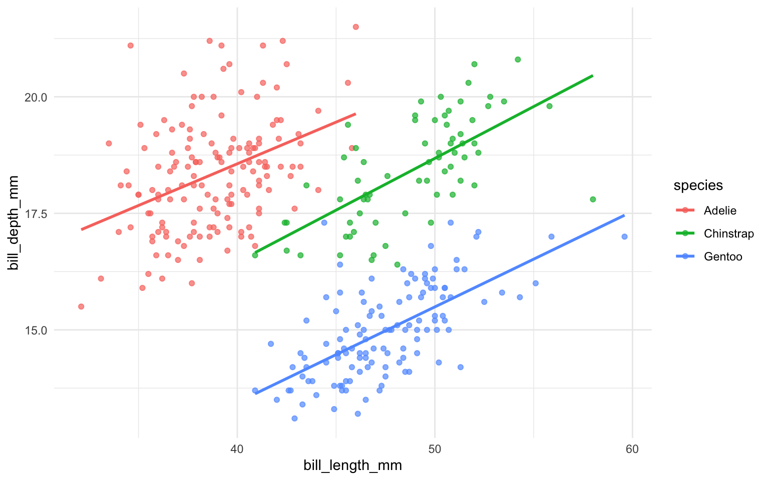
This chunk adds a neat caption and custom dimensions for the plot.
Cross-Referencing Figures
Use the fig- prefix in your label (e.g., #| label: fig-penguins) and then reference it in text with @fig-penguins. Quarto automatically numbers them for you!
17.4.2 Creating Tables
You can easily turn a tibble into a table in your document with knitr::kable(). Here’s an example:
penguins |>
    group_by(species) |>
    summarise(
        number = n(),
        mean_bill_length = mean(bill_length_mm, na.rm = TRUE),
    ) |>
knitr::kable()| species | number | mean_bill_length |
|---|---|---|
| Adelie | 152 | 38.79139 |
| Chinstrap | 68 | 48.83382 |
| Gentoo | 124 | 47.50488 |
Quarto can also display stunning tables. In R, there is a package called gt (Grammar of Tables) that makes it easy to create and style tables. Here’s an example:
| Penguins in the Palmer Archipelago | ||||||||
|---|---|---|---|---|---|---|---|---|
| Data is courtesy of the {palmerpenguins} R package | ||||||||
Adelie
|
Na |
Chinstrap
|
Gentoo
|
|||||
| Female | Male | Female | Male | Female | Male | Na | ||
| Island: Biscoe | ||||||||
| 2007 | 5 | 5 | - | - | - | 16 | 17 | 1 |
| 2008 | 9 | 9 | - | - | - | 22 | 23 | 1 |
| 2009 | 8 | 8 | - | - | - | 20 | 21 | 3 |
| Island: Dream | ||||||||
| 2007 | 9 | 10 | 1 | 13 | 13 | - | - | - |
| 2008 | 8 | 8 | - | 9 | 9 | - | - | - |
| 2009 | 10 | 10 | - | 12 | 12 | - | - | - |
| Island: Torgersen | ||||||||
| 2007 | 8 | 7 | 5 | - | - | - | - | - |
| 2008 | 8 | 8 | - | - | - | - | - | - |
| 2009 | 8 | 8 | - | - | - | - | - | - |
Check the official document and tutorial for how to create tables with gt.
17.5 Writing Equations
Quarto supports LaTeX-style math notation, which is perfect for academic writing. Use single dollar signs for inline math (e.g., $\bar{x} = \frac{1}{n}\sum x_i$ renders as \(\bar{x} = \frac{1}{n}\sum x_i\)) and double dollar signs for display math:
\[ \hat{\beta} = (X^TX)^{-1}X^Ty \]
This is especially useful when you want to show the formulas behind your statistical analyses right alongside the code that implements them.
17.6 Rendering Your Document
To turn your .qmd file into a polished document, click the Render button in RStudio (or run quarto render in the terminal). Quarto will:
- Execute all code chunks
- Capture outputs (plots, tables, printed results)
- Combine everything into your chosen format
You can switch formats just by changing the format: field in your YAML header:
format: html   # Interactive, web-friendly
format: typst  # Lightning-fast PDFs for printing and journals
format: docx   # For collaborators who love Word
The Power of Reproducibility
The beauty of Quarto is that anyone can take your .qmd file, hit Render, and get the exact same document. No more “but it works on my machine!” — your entire analysis pipeline is captured in one file.