# A tibble: 94 × 3
   Entity  Year `Annual CO₂ emissions (per capita)`
   <chr>  <dbl>                               <dbl>
 1 World   1750                              0.0124
 2 World   1760                              0.0133
 3 World   1770                              0.0158
 4 World   1780                              0.0176
 5 World   1790                              0.0216
 6 World   1800                              0.0343
 7 World   1810                              0.0384
 8 World   1820                              0.0476
 9 World   1830                              0.0775
10 World   1840                              0.0982
# ℹ 84 more rowsImport and Join Data
EE BIOL C177/C234
The here Package

Always Visualize After Import!
Sense-check: does the data look right?
data_co2 |>
  ggplot(aes(x = year, y = co2)) +
  geom_line() +
  labs(
    x = "Year",
    y = "Annual CO2 emissions per capita"
  ) +
  jtools::theme_nice()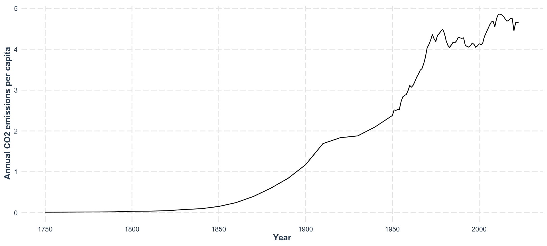
CO₂ is rising — but how does it relate to temperature? 🤔
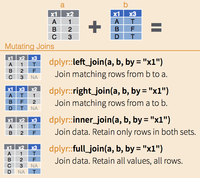
Join Types
The Payoff: CO₂ vs Temperature 🌡️
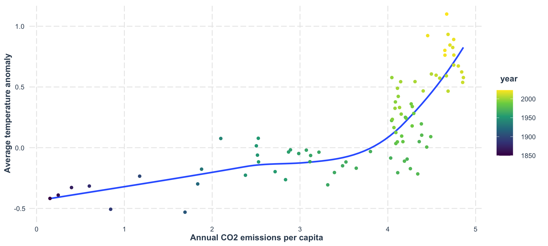
This is why we learn to join data — to answer real questions!