Five Verbs for Tidying Data

EE BIOL C177/C234

Chuliang Song

Packages for this chapter

If you haven’t installed the following packages, run this code:

pak::pak(c("tidylog", "datasauRus", "dcldata"))

Today’s Menu 🎯

1. pivot_longer() — wide → long
2. pivot_wider() — long → wide
3. separate() — split columns
4. drop_na() / replace_na() — handle missing values
5. Tidy a real dataset — the Datasaurus Dozen 🦕

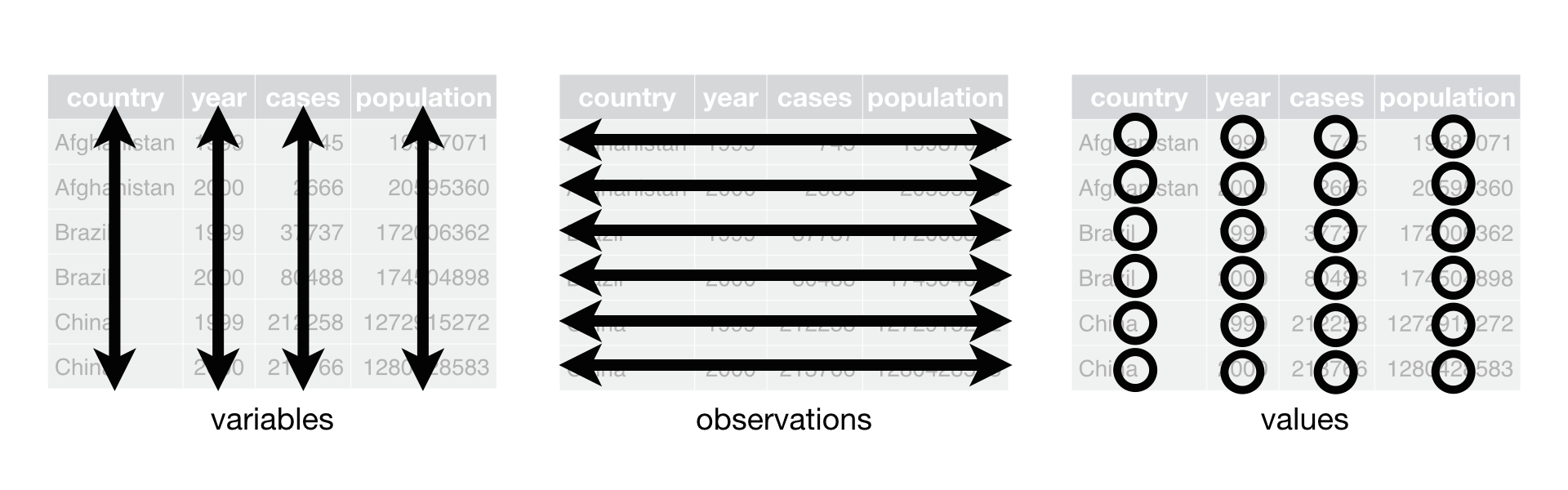
Tidy Data Reminder

Tidy datasets are all alike, but every messy dataset is messy in its own way. — Hadley Wickham

• Every row = one observation
• Every column = one variable
• Every cell = one value

From https://r4ds.hadley.nz/data-tidy.html

Why Tidy Data?

A Messy Survey Data

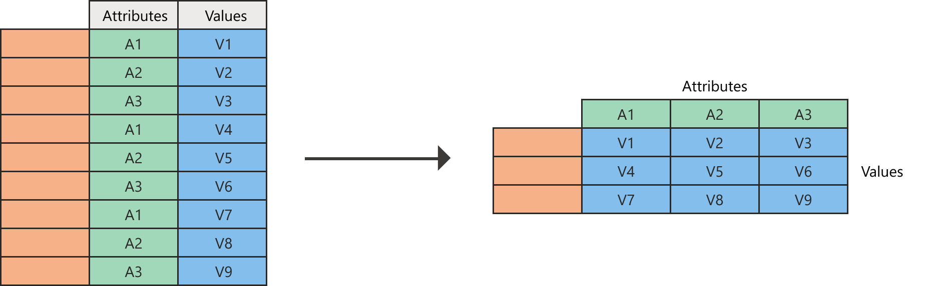
Reshaping Data

pivot_longer() — Wide to Long

library(tidyverse)
library(dcldata)
library(tidylog)
example_eagle_nests

# A tibble: 3 × 3
  region                     `2007` `2009`
  <chr>                       <dbl>  <dbl>
1 Pacific                      1039   2587
2 Southwest                      51    176
3 Rocky Mountains and Plains    200    338

Years are trapped in column names — they should be values!

pivot_longer() in Action

example_eagle_nests |>
  pivot_longer(
    cols = c(`2007`, `2009`),
    names_to = "year",
    values_to = "nests"
  )

# A tibble: 6 × 3
  region                     year  nests
  <chr>                      <chr> <dbl>
1 Pacific                    2007   1039
2 Pacific                    2009   2587
3 Southwest                  2007     51
4 Southwest                  2009    176
5 Rocky Mountains and Plains 2007    200
6 Rocky Mountains and Plains 2009    338

Conceptualizing pivot_longer()

When to use quotes?

example_eagle_nests |>
  pivot_longer(
    cols = c(`2007`, `2009`),
    names_to = "year",
    values_to = "nests"
  )

• "year" and "nests" are in quotes because they’re new columns
• We’re creating them, not referencing existing ones
• General rule: quotes when creating, no quotes when selecting

pivot_wider() — Long to Wide

The reverse of pivot_longer():

eagle_nests_longer <- example_eagle_nests |>
  pivot_longer(
    cols = c(`2007`, `2009`),
    names_to = "year",
    values_to = "nests"
  )

eagle_nests_longer |>
    pivot_wider(
        names_from = "year",
        values_from = "nests"
    )

# A tibble: 3 × 3
  region                     `2007` `2009`
  <chr>                       <dbl>  <dbl>
1 Pacific                      1039   2587
2 Southwest                      51    176
3 Rocky Mountains and Plains    200    338

When to Use Each?

Direction	Function	Use case
Wide → Long	pivot_longer()	Column names are data values
Long → Wide	pivot_wider()	Need side-by-side comparison

pivot_wider() in Practice

• Calculate the mean
• Sex as columns
• Visualize differences

We first calculate the mean bill length by group:

Because comparing values side by side is clearer, we pivot the data wider:

Splitting Columns

separate() — Split One Column

The example_gymnastics_2 dataset has combined column names:

example_gymnastics_2

# A tibble: 3 × 5
  country       vault_2012 floor_2012 vault_2016 floor_2016
  <chr>              <dbl>      <dbl>      <dbl>      <dbl>
1 United States       48.1       45.4       46.9       46.0
2 Russia              46.4       41.6       45.7       42.0
3 China               44.3       40.8       44.3       42.1

Step 1: Pivot Longer

example_gymnastics_2 |>
    pivot_longer(
        cols = -c(`country`), 
        names_to = "eventandyear", 
        values_to = "score"
    )

# A tibble: 12 × 3
   country       eventandyear score
   <chr>         <chr>        <dbl>
 1 United States vault_2012    48.1
 2 United States floor_2012    45.4
 3 United States vault_2016    46.9
 4 United States floor_2016    46.0
 5 Russia        vault_2012    46.4
 6 Russia        floor_2012    41.6
 7 Russia        vault_2016    45.7
 8 Russia        floor_2016    42.0
 9 China         vault_2012    44.3
10 China         floor_2012    40.8
11 China         vault_2016    44.3
12 China         floor_2016    42.1

Step 2: Separate the Column

example_gymnastics_2 |>
    pivot_longer(
        cols = -c(`country`), 
        names_to = "eventandyear", 
        values_to = "score"
    ) |>
    separate(
        col = "eventandyear", 
        into = c("event", "year"), 
        sep = "_"
    )

# A tibble: 12 × 4
   country       event year  score
   <chr>         <chr> <chr> <dbl>
 1 United States vault 2012   48.1
 2 United States floor 2012   45.4
 3 United States vault 2016   46.9
 4 United States floor 2016   46.0
 5 Russia        vault 2012   46.4
 6 Russia        floor 2012   41.6
 7 Russia        vault 2016   45.7
 8 Russia        floor 2016   42.0
 9 China         vault 2012   44.3
10 China         floor 2012   40.8
11 China         vault 2016   44.3
12 China         floor 2016   42.1

💡 unite() — The Reverse of separate()

unite() combines multiple columns into one:

tibble(
  month = c(1, 2, 3),
  day = c(15, 20, 25),
  year = c(2020, 2020, 2020)
) |>
  unite(
    col = "full_date",
    month, day, year,
    sep = "-"
  )

# A tibble: 3 × 1
  full_date
  <chr>    
1 1-15-2020
2 2-20-2020
3 3-25-2020

Missing Values

drop_na() — Remove Missing Rows

library(palmerpenguins)
penguins |> 
  drop_na()

# A tibble: 333 × 8
   species island    bill_length_mm bill_depth_mm flipper_length_mm body_mass_g
   <fct>   <fct>              <dbl>         <dbl>             <int>       <int>
 1 Adelie  Torgersen           39.1          18.7               181        3750
 2 Adelie  Torgersen           39.5          17.4               186        3800
 3 Adelie  Torgersen           40.3          18                 195        3250
 4 Adelie  Torgersen           36.7          19.3               193        3450
 5 Adelie  Torgersen           39.3          20.6               190        3650
 6 Adelie  Torgersen           38.9          17.8               181        3625
 7 Adelie  Torgersen           39.2          19.6               195        4675
 8 Adelie  Torgersen           41.1          17.6               182        3200
 9 Adelie  Torgersen           38.6          21.2               191        3800
10 Adelie  Torgersen           34.6          21.1               198        4400
# ℹ 323 more rows
# ℹ 2 more variables: sex <fct>, year <int>

drop_na() — Targeting Specific Columns

You can drop NAs in just one column:

penguins |>
  drop_na(bill_length_mm)

# A tibble: 342 × 8
   species island    bill_length_mm bill_depth_mm flipper_length_mm body_mass_g
   <fct>   <fct>              <dbl>         <dbl>             <int>       <int>
 1 Adelie  Torgersen           39.1          18.7               181        3750
 2 Adelie  Torgersen           39.5          17.4               186        3800
 3 Adelie  Torgersen           40.3          18                 195        3250
 4 Adelie  Torgersen           36.7          19.3               193        3450
 5 Adelie  Torgersen           39.3          20.6               190        3650
 6 Adelie  Torgersen           38.9          17.8               181        3625
 7 Adelie  Torgersen           39.2          19.6               195        4675
 8 Adelie  Torgersen           34.1          18.1               193        3475
 9 Adelie  Torgersen           42            20.2               190        4250
10 Adelie  Torgersen           37.8          17.1               186        3300
# ℹ 332 more rows
# ℹ 2 more variables: sex <fct>, year <int>

Only removes rows where bill_length_mm is NA

replace_na() — Fill Missing Values

penguins |>
  replace_na(
    list(sex = "male")
  )

# A tibble: 344 × 8
   species island    bill_length_mm bill_depth_mm flipper_length_mm body_mass_g
   <fct>   <fct>              <dbl>         <dbl>             <int>       <int>
 1 Adelie  Torgersen           39.1          18.7               181        3750
 2 Adelie  Torgersen           39.5          17.4               186        3800
 3 Adelie  Torgersen           40.3          18                 195        3250
 4 Adelie  Torgersen           NA            NA                  NA          NA
 5 Adelie  Torgersen           36.7          19.3               193        3450
 6 Adelie  Torgersen           39.3          20.6               190        3650
 7 Adelie  Torgersen           38.9          17.8               181        3625
 8 Adelie  Torgersen           39.2          19.6               195        4675
 9 Adelie  Torgersen           34.1          18.1               193        3475
10 Adelie  Torgersen           42            20.2               190        4250
# ℹ 334 more rows
# ℹ 2 more variables: sex <fct>, year <int>

⚠️ Always be explicit about how you handle NAs!

A cautionary tale: bad NA handling retracted a Nature paper

Putting It All Together

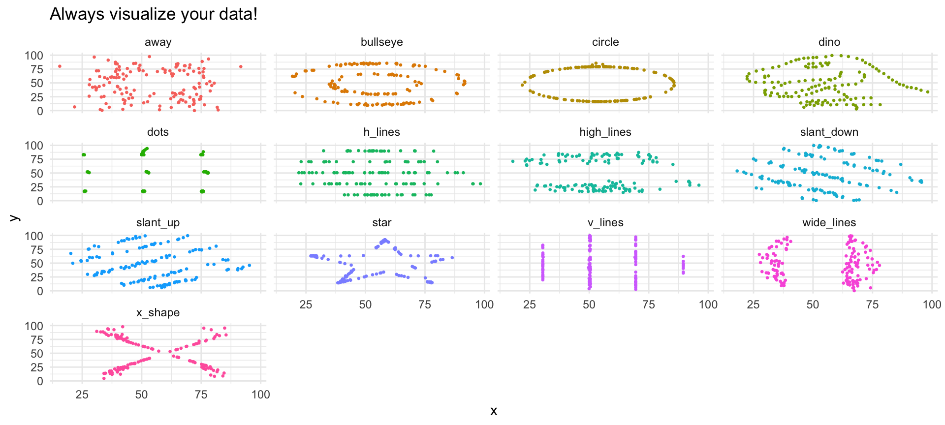
The Datasaurus Dozen 🦕

Can you trust summary statistics alone?

library(datasauRus)
datasaurus_dozen_wide

Let’s tidy this dataset using everything we learned today!

Step 1: Pivot Longer

library(datasauRus)
datasaurus_dozen_long <- datasaurus_dozen_wide |>
  mutate(row = row_number()) |>
  pivot_longer(
    cols = -"row",
    names_to = "variable",
    values_to = "value"
  )

Add a row ID, then pivot all columns to long format

Step 2: Separate + Pivot Wider

datasaurus <- datasaurus_dozen_long |>
  separate(
    variable, 
    into = c("dataset", "coord"),
    sep = "_(?=[^_]*$)"
  ) |>
  pivot_wider(
    names_from = "coord", values_from = "value"
  )

Split at the last underscore, then spread x/y into columns

Same Statistics…

datasaurus |>
  group_by(dataset) |>
  summarise(
    mean_x = mean(x), mean_y = mean(y),
    sd_x = sd(x), sd_y = sd(y),
    cor = cor(x, y)
  )

# A tibble: 13 × 6
   dataset    mean_x mean_y  sd_x  sd_y     cor
   <chr>       <dbl>  <dbl> <dbl> <dbl>   <dbl>
 1 away         54.3   47.8  16.8  26.9 -0.0641
 2 bullseye     54.3   47.8  16.8  26.9 -0.0686
 3 circle       54.3   47.8  16.8  26.9 -0.0683
 4 dino         54.3   47.8  16.8  26.9 -0.0645
 5 dots         54.3   47.8  16.8  26.9 -0.0603
 6 h_lines      54.3   47.8  16.8  26.9 -0.0617
 7 high_lines   54.3   47.8  16.8  26.9 -0.0685
 8 slant_down   54.3   47.8  16.8  26.9 -0.0690
 9 slant_up     54.3   47.8  16.8  26.9 -0.0686
10 star         54.3   47.8  16.8  26.9 -0.0630
11 v_lines      54.3   47.8  16.8  26.9 -0.0694
12 wide_lines   54.3   47.8  16.8  26.9 -0.0666
13 x_shape      54.3   47.8  16.8  26.9 -0.0656

…Completely Different Shapes!

datasaurus |>
  ggplot(aes(x, y, color = dataset)) +
  geom_point(size = 0.5) +
  facet_wrap(vars(dataset)) +
  theme_minimal() +
  theme(legend.position = "none") +
  labs(title = "Always visualize your data!")

Summary

• pivot_longer() / pivot_wider() reshape data
• separate() splits, unite() combines columns
• drop_na() removes, replace_na() fills missing values
• The Datasaurus shows: never trust summaries alone — always visualize!